Equation Overview - Rotation and Balance
NOTE: The original CalcPad unit for Rotation was split into 3 subpages and had equations for each. This is now combined onto this page. Please use the links below or the page level navigation to skip to the appropriate equations overview. Additionally, this page existed before we had our Balance and Rotation tutorial written, so the contents here go beyond a summary. We apologize for the length of this page.
Equation Overview - Rotational Kinematics (RK)
Problem Set Overview
We have 8 ready-to-use problem sets on the topic of Rotational Kinematics. These problem sets focus on the analysis of situations involving a rigid object rotating in either a clockwise or counterclockwise direction about a given point. The object's rotation speed may be increasing, decreasing, or remaining constant.
Characteristics of Objects in Rotational Motion
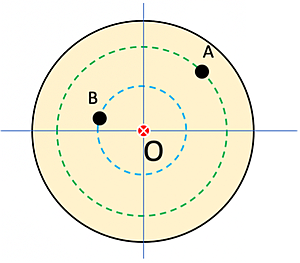
Objects in purely rotational motion involve rigid (non-deformable) objects that have a singular point around which all other points on the object complete a circular path in one complete rotation of the object. Consider Point O to be the axis of rotation in the object at right. Points A and B will follow the dotted circular paths if the object is rotated.
Angular Position and Angular Displacement
Consider the initial position of a point at position A on the x-axis as shown below left. After a period of time the point has rotated counterclockwise to its new position B shown below right. The point is now at an angular position of θ with reference to the x-axis. That angular position can be described in units of degrees or radians.
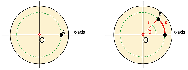
The radian is an angular measure that is defined by the ratio of the arc length traveled, s, divided by the radius, r, expressed as an equation, it can be said θ = s/r.
There are 360˚ or 2π radians in a full circle. Therefore,
\(1 \text{Radian} = \frac{360°}{2π} = 57.3°\)
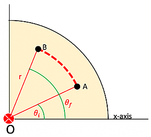
If a point is rotated around a fixed center on a rigid body from an initial position, A, to a final position, B, we say it has had an angular displacement. That would be evaluated as:
\(\text{δt} = θ_f - θ_i\) SI Unit: Radian
The quantity \(\text{δθ}\) would have a positive value if displaced counterclockwise and a negative direction if displaced clockwise.
Average and Instantaneous Angular Velocity
If a point is rotated around a fixed center on a rigid body from an initial angular position to a final angular position over a period of time, we say it has an average angular velocity, \(ω_\text{avg}\). That value would be evaluated as \(ω_\text{avg} = \text{δθ} \div \text{δt}\). A positive or negative calculation result would depend on the sign of \(\text{δθ}\). The average angular speed would be the magnitude of the average angular velocity.
The instantaneous angular velocity of a rotating rigid object is mathematically defined as the limit of the average speed as the time interval \(\text{δt}\) approaches zero:
\(ω = \underset{\text{δt} \to 0}{\text{lim}} \frac{\text{δθ}}{\text{δt}}\) SI unit radian/sec
The instantaneous angular speed is the magnitude of the instantaneous angular velocity. When the angular speed is constant, the instantaneous angular speed is equal to the average angular speed.
Average and Instantaneous Angular Acceleration
If a point is rotated around a fixed center on a rigid body with an initial angular velocity, \(ω_i\), to a final angular velocity, \(ω_i\), over a period of time, we say it has an average angular acceleration, \(a_\text{avg}\). That value would be evaluated as \(a_\text{avg} = \text{δω} \div \text{δt}\). A positive or negative calculation result would depend on the sign of \(\text{δω}\).
The instantaneous angular acceleration of a rotating rigid object is mathematically defined as the limit of the average acceleration as the time interval \(\text{δt}\) approaches zero:
\(α = \underset{\text{δt} \to 0}{\text{lim}} \frac{\text{δω}}{\text{δt}}\) SI unit: radian/sec2
When the angular acceleration is constant, the instantaneous angular acceleration is equal to the average angular acceleration.
Rotational Motion under Constant Angular Acceleration
The definitions for the rotational quantities, \(θ\), \(\text{δθ}\), \(ω\), \(\text{δω}\), and \(α\) are similar to the definitions for the linear quantities, \(x\), \(\text{δx}\), \(v\), \(\text{δv}\), and \(a\). Due to the rotational variables sharing the same mathematical relationships between them as the linear variables, new equations can be written for rotational motion that mimic the equations for linear motion.
The comparison of equations for Linear Motion with a constant acceleration, and their counterpart Rotational motion equations with a constant linear acceleration (alpha)
Linear Motion with a Constant
Linear Motion with α Constant
\(v = v_o + a \times t\)
\(ω = ω_o + α \times t\)
\(\text{δx} = ½ \times (v_o + v) \times t\)
\(\text{δθ} = ½ \times (ω_o + ω) \times t\)
\(\text{δx} = v_o \times t + ½ \times a \times t^2\)
\(\text{δθ} = ω_o \times t + ½ \times α \times t^2\)
\(v^2 = v_o^2 + 2 \times a \times \text{δx}\)
\(ω^2 = ω_o^2 + 2 \times α \times \text{δθ}\)
Every term in a specific linear equation has a corresponding term in the analogous rotational equation.
Relations between Angular and Linear Quantities
Consider a point P on an arbitrarily shaped, rigid object able to rotate counterclockwise around an axis of rotation at O in the z-direction. The point P starts on the x-axis at a radial distance of r and ends at the position shown below. That point will have rotated through an angular displacement, \(\text{δθ}\)), and an arc length, \(\text{δs}\)).
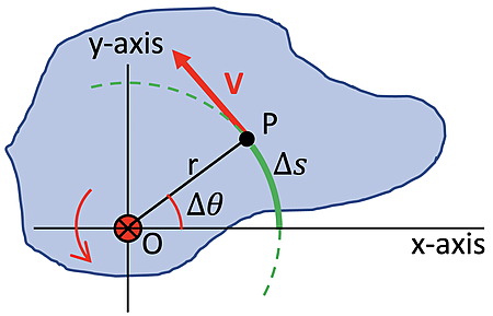
The relationship between \(r\), \(\text{δθ}\), and \(\text{δs}\) is the following:
\(\text{δθ} = \frac{\text{δs}}{r}\)
If the time interval to complete the rotation is \(\text{δt}\), dividing both sides by this increment of time gives:
\(\frac{\text{δθ}}{\text{δt}} = \frac{1}{r} \times \frac{\text{δs}}{\text{δt}}\)
As the time interval, \(\text{δt}\), approaches zero, the ratio on the left approaches the instantaneous angular velocity, \(ω\), and the ratio on the right approaches the linear velocity, \(v\), that becomes tangent to the curve. Performing these substitutions gives:
\(ω = \frac{v}{r}\) - or - \(v = ω \times r\)
If point P started from rest, it experienced a change in angular and linear speed as it rotated from its original position. We can analyze this situation by dividing the previous equation by the time interval, \(\text{δt}\).
\(\frac{\text{δω}}{\text{δt}} = \frac{1}{r} \times \frac{\text{δv}}{\text{δt}}\)
Once again as the time interval, \(\text{δt}\), approaches zero, the ratio on the left approaches the instantaneous angular acceleration, \(α\), and the ratio on the right approaches the linear acceleration, \(a\), that becomes tangent to the curve. Performing these substitutions gives:
\(α = \frac{1}{r} \times a_\text{tan}\) - or - \(a_\text{tan} = α \times r\)
Summary of Conditions for Kinematic Rotational Motion
One difficulty a student may encounter with this topic is the confusion as to which formula to use. When approaching these problems it is suggested that you practice the usual habits of an effective problem-solver; identify known and unknown quantities in the form of the symbols of physics formulas, plot out a strategy for using the knowns to solve for the unknown, and then finally perform the necessary algebraic steps and substitutions required for the solution.
Three equations that show the relationships between linear motion (distance, velocity, acceleration) and rotational motion (angular displacement, angular velocity, angular acceleration with respects to radius r)
Linear and Rotational Relationship
\(\text{δs} = \text{δθ} \times r\)
\(v_\text{tan} = ω \times r\)
\(a_\text{tan} = α \times r\)
The big four equations for rotational motion
Rotational Big 4
\(ω = ω_o + α \times t\)
\(\text{δθ} = ½ \times (ω_o + ω) \times t\)
\(\text{δθ} = ω_o \times t + ½ \times α \times t^2\)
\(ω^2 = ω_o^2 + 2 \times α \times \text{δθ}\)
Habits of an Effective Problem-Solver
An effective problem solver by habit approaches a physics problem in a manner that reflects a collection of disciplined habits. While not every effective problem solver employs the same approach, they all have habits which they share in common. These habits are described briefly here. An effective problem-solver...
- ...reads the problem carefully and develops a mental picture of the physical situation. If needed, they sketch a simple diagram of the physical situation to help visualize it.
- ...identifies the known and unknown quantities in an organized manner, often times recording them on the diagram itself. They equate given values to the symbols used to represent the corresponding quantity (e.g., \(\text{δθ} = \units{0.982}{\text{rad}}\), \(ω_o = \units{0.0}{\frac{\text{rads}}{s}}\), \(r = \units{0.251}{m}\), \(ω = \colorbox{gray}{Unknown}\)).
- ...plots a strategy for solving for the unknown quantity. The strategy will typically center around the use of physics equations and is heavily dependent upon an understanding of physics principles.
- ...identifies the appropriate formula(s) to use, often times writing them down. Where needed, they perform the needed conversion of quantities into the proper unit.
- ...performs substitutions and algebraic manipulations in order to solve for the unknown quantity.
Equation Overview - Rotation and Torque
Problem Set Overview
There are 14 ready-to-use problem sets on the topic of Rotation and Torque. The problems target your ability to use analyze a beam in terms of torque in order to determine the conditions for which it will and will not rotate.
Characteristics of Objects in Static Equilibrium
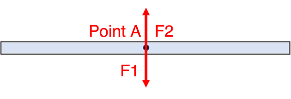
Objects in static equilibrium may experience forces in 2 perpendicular dimensions. Two of the three conditions that must be satisfied to make it a static situation are that \(\sum{F} = 0 N\) in both of those directions. For example, in the diagram below the magnitude of F1 is equal to the magnitude of F2 and the object can remain at rest since adding the 2 force vectors gives a zero net force.
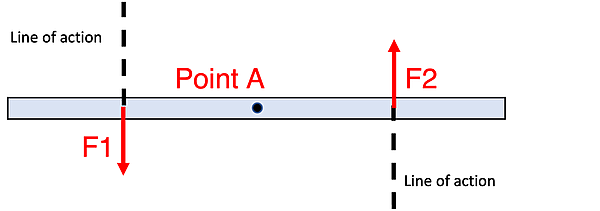
An issue that challenges static equilibrium arises when forces don’t share the same line of action (black dotted lines) as they did above. In the case below \(\sum{F} = 0 N\) is valid in the vertical direction, but since the position of F1 and F2 are offset from each other the object would rotate around Point A in a counterclockwise direction. We say that these forces individually will cause a torque, and since both try to rotate the object counterclockwise, they will produce a net torque resulting in rotation, about point A.
Mathematical Analysis of Objects Experiencing Torques
In order to analyze the torque on an object mathematically we use the definition of the torque vector cross product equation: \(τ = r \times F\) where the symbol τ (Greek letter tau, pronunciation) represents Torque. This mathematical analysis of torque is heavily dependent upon an understanding of the vector cross product between r (position vector from Point A to the position of force applied) and F (force vector on the object) in the definition. The operation of the mathematical cross product creates a third vector perpendicular to the original 2 vectors using the right-hand rule as shown below. The index finger points in the direction of r, the middle finger curls into the direction of F, and the thumb points in the direction of τ. If r and F are in the x-y plane the torque vector, τ would be in the z axis direction.
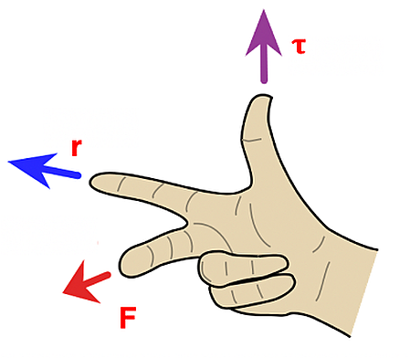
Image Credit https://commons.wikimedia.org/wiki/File:Right_hand_rule_cross_product.svg
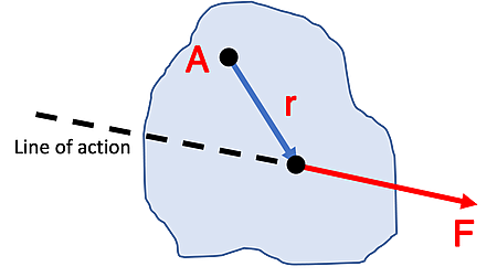
To see how to calculate a value of the torque vector let’s consider the single force, F, on the generic object below with a pin joint present at point A (this will be the axis of rotation on a line in and out of the page). Since the force, F, does not lie on a line of action passing through point A it will rotate the object about that point.
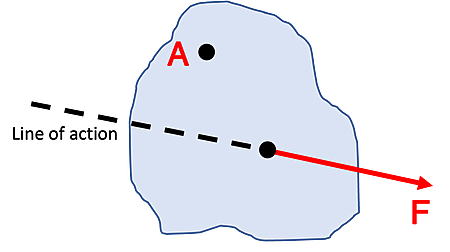
The position vector, r, connects the axis of rotation (Point A) to the point at which the force is applied to the object as shown below.
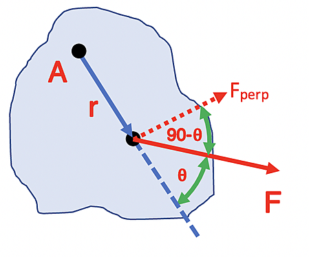
The evaluation of the vector cross product using r and F in an algebraic calculation is shown below left. The relationship of r, F, and θ relative to point A is shown below right.
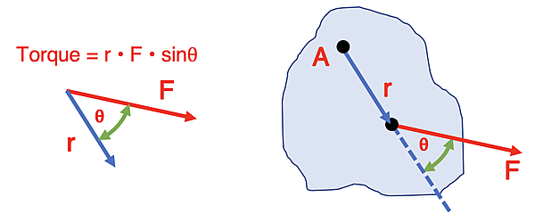
\(\text{Torque} = r \times F \times \sin{θ}\)
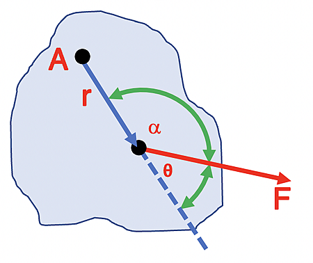
An equivalent evaluation of the cross product would be to use the angle, α, as shown below. This angle is supplementary to θ so the value of \(r \times F \times \sin{α}\) will produce the same value as the previous method since the 2 angles will produce the same sine value.
Other ways to Complete the Vector Cross Product Calculation
There are other ways to evaluate the cross product. One is to use a perpendicular distance from the axis point (Point A) to the line of action of the force as shown below (blue dotted line). This perpendicular distance is sometimes called the "lever arm" or "moment arm". The torque value will then be \(\text{lever arm} \times \text{Force}\) and evaluate to be \(r \times \sin{θ} \times F\). This would produce the same value as the previous method.
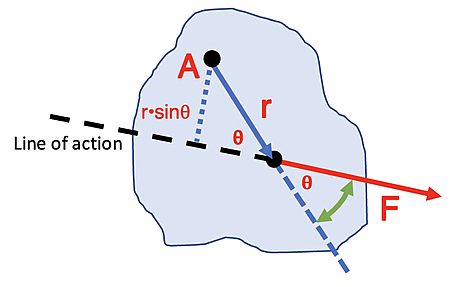
"Lever Arm": \(r \times \sin{θ}\)
Another way would be to use the component of F perpendicular to the position vector, r, as shown below. The torque would be evaluated as \(r \times F_\text{perp}\) which is equal to \(r \times F \times \cos{(90 - θ)}\) that once again would produce the same value as \(r \times F \times \sin{θ}\).
Net Torque and Direction
The goal of the Torque analysis is to determine the magnitude of all torque values from individual forces that are on lines of action not passing through the chosen axis of rotation point. These will then determine the overall torque (Net Torque or \(\sum{τ}\)) upon the object.
We can more easily conceptualize this analysis by determining whether the force vectors are trying to rotate the object clockwise or counterclockwise in the plane of the position vector, r, and force vector, F, about the point chosen. We would then proceed by adding all the torque values in the counterclockwise direction and subtracting all torques in the clockwise direction. If this sum is equal to 0 then the third condition for static equilibrium is satisfied: \(\sum{τ} = 0\).
Summary of Conditions for Static Equilibrium
One difficulty a student may encounter with this topic is the confusion as to which formula to use. The table below provides a useful summary of the formulae pertaining to torque and rotary motion. When approaching these problems it is suggested that you practice the usual habits of an effective problem-solver; identify known and unknown quantities in the form of the symbols of physics formulas, plot out a strategy for using the knowns to solve for the unknown, and then finally perform the necessary algebraic steps and substitutions required for the solution.
x direction: \(\sum{F_x} = 0\)
y direction: \(\sum{F_y} = 0\)
Any point chosen: \(\sum{τ} = 0\)
Habits of an Effective Problem-Solver
An effective problem solver by habit approaches a physics problem in a manner that reflects a collection of disciplined habits. While not every effective problem solver employs the same approach, they all have habits which they share in common. These habits are described briefly here. An effective problem-solver...
- ...reads the problem carefully and develops a mental picture of the physical situation. If needed, they sketch a simple diagram of the physical situation to help visualize it.
- ...identifies the known and unknown quantities in an organized manner, often times recording them on the diagram itself. They equate given values to the symbols used to represent the corresponding quantity (e.g., \(m = \units{1.50}{\text{kg}}\), \(F = \units{12.2}{N}\), \(r = \units{0.133}{m}\), \(Torque = \colorbox{gray}{Unknown}\)).
- ...plots a strategy for solving for the unknown quantity. The strategy will typically center around the use of physics equations and is heavily dependent upon an understanding of physics principles.
- ...identifies the appropriate formula(s) to use, often times writing them down. Where needed, they perform the needed conversion of quantities into the proper unit.
- ...performs substitutions and algebraic manipulations in order to solve for the unknown quantity.
Equation Overview - Rotational Dynamics
Problem Set Overview
There are 8 ready-to-use problem sets on the topic of Rotational Dynamics. These problem sets focus on the analysis of situations involving a rigid object or objects rotating in either a clockwise or counterclockwise direction about a given point. The object's rotation speed may be increasing, decreasing, or remaining constant.
Derivation of Net Torque Equation
Consider an object of mass, m, on a horizontal surface connected by a massless rod to a center point O. A force, F, tangent to a circle of radius, r, is applied to the mass without frictional effects as shown below.
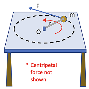
* We know that a circular motion requires an inward or centripetal force. In this derivation, our focus is on the effect of the tangential force. Since the centripetal force does not affect tangential force, we are not including it in this discussion.
Since the motion we care about is in the horizontal plane, we can ignore the gravitational and normal force on the mass. The equation using Newton’s 2nd Law in the tangential direction would be \(F = m \times a\).
Therefore,
\(F_\text{tan} = m \times a_\text{tan}\)
Multiplying both sides by r:
\(f_\text{tan} \times r = m \times r \times a_\text{tan}\)
Substituting from Rotational Kinematics:
\(a_\text{tan} = r \times α\)
Using the definition for torque: \(τ = r \times F\), which is just the left side, then,
\(τ = m \times r^2 \times α\)
This reveals that the torque on an object is directly related to the angular acceleration of the object, \(τ \times a\), with the constant of proportionality being \(m \times r^2\). This constant of proportionality can also be thought of as the resistance to angular acceleration. This constant of proportionality or resistance to a change in motion is called the Moment of Inertia, I.
The final equation is
\(τ = I \times α\)
where \(I = m \times r^2\) for an object (considered a point mass) going around a center point at a constant radius.
Moment of Inertia for Other Objects
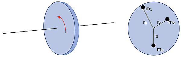
The question arises as to what the moment of inertia, I, would be if all of the mass wasn’t concentrated at the same radius. Let’s use a solid disk and consider it to be made up of many point masses at many different radii as shown in the image below.
The net torque on the disk is given by the sum of the individual torques on all the particles:
\(\sum{τ} = (\sum{m \times r^2}) \times α\)
Since all of the mass particles have the same angular acceleration the moment of inertia for a solid disk is
\(\sum{m \times r^2}\) - SI Unit: kg·m2
Using calculus, not shown here, the moment of inertia for a solid disk of radius, R, and mass, M, is
\(I_\text{disk} = ½ \times M \times R^2\)
Moments of inertia for common objects of mass, M, without proof are listed below.
Moments of Inertia for Common objects, with their name, image, and Inertia equation
Object
Drawing
Inertia Equation
Hoop or Think Cylindrical Shell
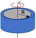
Thickness of the ring is small relative to its inner radius.
\(M \times R^2\)
Solid Cylinder or Disk
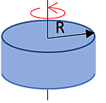
\(½ \times M \times R^2\)
Long Thin Rod Rotation Axis through Center
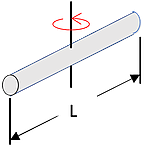
\(\frac{1}{12} \times M \times L^2\)
Long Thin Rod Rotation Axis through End
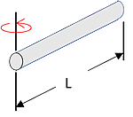
\(⅓ \times M \times L^2\)
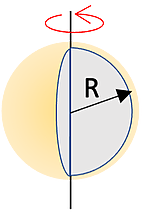
Solid Sphere
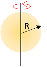
\(\frac{2}{5} \times M \times R^2\)
Hollow Spherical Shell
Thickness of the shell is small relative to its inner radius.
\(\frac{2}{3} \times M \times R^2\)
Moment of Inertia for Composite Objects
Consider an object that is made up of more fundamental objects as depicted in the previous table. For example, let’s look at a baton that is twirled in the middle consisting of a thin rod (mass M), and a point mass, m, on each end as shown below.
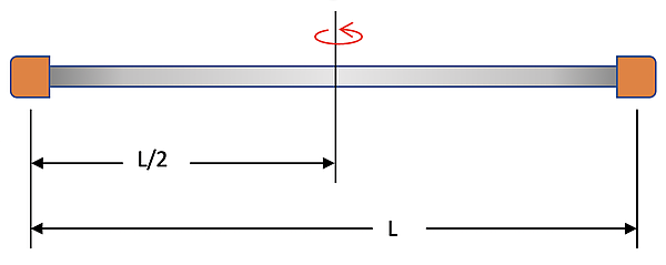
The total resistance to rotation around the vertical center line has to include the rod and the 2-point masses to get the total Moment of Inertia for the system.
\(I_\text{total} = I_\text{rod} + I_\text{left point mass} + I_\text{right point mass}\)
\(I_\text{total} = \frac{1}{12} \times M \times L^2 + M \times (\frac{L}{2})^2 + M \times (\frac{L}{2})^2\)
\(I_\text{total} = \frac{7}{12} \times M \times L^2\)
Moments of Inertia about an Unusual Axis
Consider an object that is rotating around an axis that does not go through the center of mass of the object. An example would be twirling a long, thin rod around an axis that is ¼ of the way from the center of mass. To determine this Moment of Inertia we use the Parallel Axis Theorem that states:
The Moment of Inertia of an object of mass, M, about an axis a distance, d, from the center of mass and parallel to an axis going through the center of mass is calculated by the following:
\(I_\text{parallel axis} = I_\text{center of mass} + M \times d^2\)
Let’s use the long, thin rod as shown below to calculate I about the axis through Point B. The axis through Point A is going through the center of mass.
Two images showing calculation of the Moment of Inertia through a rod at the center, and then again through a point part way down the rod.
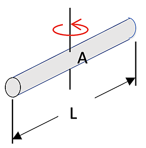
Moment of Inertia
\(I_A = I_\text{center of mass} = \frac{1}{12} \times M \times L^2\)
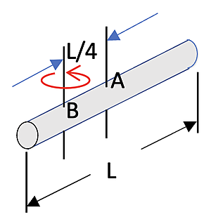
Moment of Inertia for Point B:
\(I_B = I_A + M \times (\frac{L}{4})^2\)
\(I_B = \frac{1}{12} \times M \times L^2 + \frac{1}{16} \times M \times L^2\)
\(I_B = \frac{7}{48} \times M \times L^2\)
Rotational Dynamics Equations
We can now combine the Angular and Linear Kinematics Equations with the Cause of Acceleration Equations.
Showing causes of acceleration and kinematic equations for Linear and rotational motion, with additional connecting to linear to angular equations
Linear Motion with a Constant
Connecting Linear to Angular
Linear Motion with α Constant
Cause of Acceleration
\(F_\text{net} = m \times a\)
Empty
\(τ_\text{net} = I \times α\)
Kinematic Equations
\(v = v_o + a \times t\)
\(\text{δx} = ½ \times (v_o + v) \times t\)
\(\text{δx} = v_o \times t + ½ \times a \times t^2\)
\(v^2 = v_o^2 + 2 \times a \times \text{δx}\)
\(\text{δs} = r \times \text{δθ}\)
\(v = r \times ω\)
\(a = r \times α\)
\(ω = ω_o + α \times t\)
\(\text{δθ} = ½ \times (ω_o + ω) \times t\)
\(\text{δθ} = ω_o \times t + ½ \times α \times t^2\)
\(ω^2 = ω_o^2 + 2 \times α \times \text{δθ}\)
Derivation of Rotational Kinetic Energy
Consider an object of mass, m, on a horizontal surface connected by a massless rod to a center point O. The mass has a constant speed in the tangential direction to a circle of radius, r. Shown Below.
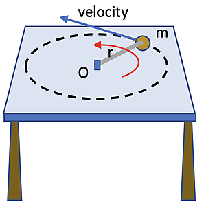
In solving Mechanics problems, it can be advantageous to analyze motion using an Energy approach. The Kinetic Energy of the mass would be as shown below:
\(KE = ½ \times m \times v_\text{tan}^2\)
Since \(v_\text{tan} = r \times ω\), this could be written as
\(KE = ½ \times m \times r^2 \times ω^2\)
And since \(I = m \times r^2\) for a point mass the Kinetic Energy of this mass rotating around a center point could be written as
\(KE = ½ \times I \times ω^2\)
What if the object was more than just a single point mass? Consider the 3 different point masses shown in the rotating solid disk around Point O at right. In order to determine their total Kinetic Energy you would have to sum them up individually as shown below:
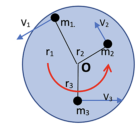
\(\text{KE} = ½ \times m_1 \times v_1^2 + ½ \times m_2 \times v_2^2 + ½ \times m_3 \times v_3^2\)
Since all point masses have the same rotational speed, \(ω\), and since \(v = r \times ω\), this could be written as
\(\text{KE} = ½ \times m_1 \times r_1^2 \times ω_1^2 + ½ \times m_2 \times r_2^2 \times ω_2^2 + ½ \times m_3 \times r_3^2 \times ω_3^2\)
leading to
\(\text{KE} = ½ \times (\sum{m \times r^2}) \times ω^2\)
If i particles in the disk are considered as i goes to infinity then \(\sum{m \times r^2} = I_\text{disk}\). The Kinetic Energy for the disk can then be written as
\(\text{KE} = ½ \times I_\text{disk} \times ω^2\)
The Kinetic Energy for any other object rotating around an axis with rotational speed, \(ω\), and moment of inertia, \(I\), can be written as
\(\text{KE} = ½ \times I \times ω^2\)
Kinetic Energy of Rolling Objects
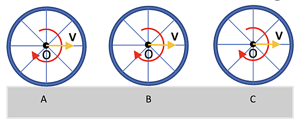
How would you determine the Kinetic Energy for an object that is rotating and translating? Let’s look at the ring moving from Position A to Position C as it rolls along the surface as shown at right. It has rotational speed, ω, around Point O, horizontal center of mass speed, v, and radius, r.
Let’s analyze the motion from the center of mass position, Point O. There would be the rotational Kinetic Energy, and since point O is moving relative to the horizontal surface, there would have to be translational Kinetic Energy as well:
\(\sum{\text{KE}} = \text{KE}_\text{rotation} + \text{KE}_\text{translation}\)
\(\sum{\text{KE}} = ½ \times I \times ω^2 + 1/2 \times m \times v^2\)
Since \(ω^2 = \frac{v^2}{r^2}\) then it can be written as
\(\sum{\text{KE}} = ½ \times m \times r^2 \times \frac{v^2}{r^2} + ½ \times m \times v^2\)
Therefore, the total (translational plus rotational) Kinetic Energy for the rolling ring is \(\text{KE} = m \times v^2\).
A way to check that result would be to calculate the rotational Kinetic Energy around a point of contact between the ring and the horizontal surface, Point A, as shown below. This will result in the rotational speed, ω, around Point A as depicted by the red arrow.
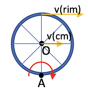
\(I_A = I_O + m \times d^2 = m \times r^2 + m \times r^2 = 2 \times m \times r^2\)
The total Kinetic Energy would be rotational only as the ring is rotating around point A at this instant and not translating (the point of contact on the ring is not moving relative to Point A on the horizontal surface).
Therefore, \(\text{KE} = ½ \times I_A \times ω^2\). and since \(ω = v_\text{cm} \div r\), then
\(\text{KE} = ½ \times (2 \times m \times r^2) \times (\frac{v_\text{cm}}{r})^2\)
v_\text relative to Point A in this case is the same as the previous horizontal center of mass speed, v, relative to the horizontal surface. In both cases then the answer to the original question (How would you determine the Kinetic Energy for an object that is rotating and translating?) is
\(\text{KE} = m \times v^2\)
Angular Momentum
In the linear case momentum (\(p = m \times v\)) was used to analyze objects in motion. When doing that it was necessary to determine if the system experienced a net external force that would cause a change in momentum. If the system did not experience a net external force the system was said to be isolated resulting in the total momentum of the system being conserved (\(\sum{p_\text{initial}} = \sum{p_\text{final}}\)).
In a similar way angular momentum can be used to analyze objects rotating around an axis. Angular momentum, L, can be defined as \(L = I \times ω\). Consider the definitions for torque and angular acceleration;
\(τ = I \times α\) - and - \(α = \frac{\text{δθ}}{\text{δt}}\)
then using substitution to get
\(τ = I \times \frac{\text{δθ}}{\text{δt}}\)
and finally multiplying each side by \(\text{δθ}\) giving the result
\(τ \times \text{δt} = I \times \text{δω} = \text{δL}\)
Thus, a change in angular momentum occurs if a net external torque acts on the system over a period of time. If the net external torque = 0, then the system is said to be isolated resulting in the total angular momentum of the system being conserved (\(\sum{L_\text{initial}} = \sum{L_\text{final}}\)), similar to the case in the linear situation.
Particle Angular Momentum
Consider an object of mass, m, on a horizontal surface connected by a massless rod to a center point O as shown below. The mass has a constant speed in the tangential direction to a circle of radius, r.
The angular momentum of the point mass would be
\(L = I \times ω\)
Substituting for I and ω gives
\(L = m \times r^2 \times \frac{v_\text{tan}}{r} = m \times r \times v_\text{tan}\)
This is the magnitude of the vector cross product for the angular momentum of a particle about the vertical axis through Point O;
\(\overrightarrow{L} = \overrightarrow{r} \times \overrightarrow{p}\)
To see how to calculate a value of the angular momentum vector in general for a point mass let’s consider the point mass below having a momentum, p, with an axis of rotation through point A (this will be a line in and out of the page). Since the linear momentum, p, does not lie on a line of action passing through point A it will produce an angular momentum about that point at this instant.
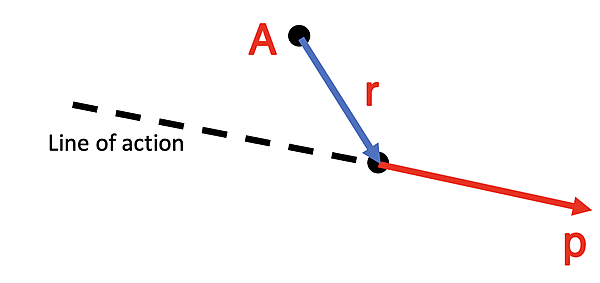
The evaluation of the vector cross product using r and p in an algebraic calculation is shown below left. The relationship of r, p, and relative to point A is shown below right.
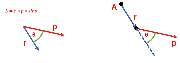
\(L = r \times p \times \sin{θ}\)
Therefore, the angular momentum at this instant would evaluate to
\(L_\text{point mass} = r \times m \times v \times \sin{θ}\)
Rotational Dynamics Equations for Momentum
We can now combine the linear momentum case and the angular momentum case.
Linear Momentum and Angular Momentum equations by the system (Point mass, solid objects, isolated system, and non-isolated system)
Linear Momentum
Angular Momentum
Point Mass
\(p = m \times v\)
\(L = r \times m \times v \times \sin{θ}\)
Solid Object
\(p_\text{cm} = m \times v_\text{cm}\)
\(L = I \times ω\)
Isolated System
\(\text{External F}_\text{net} =0\)
\(P_\text{initial} = p_\text{final}\)
\(\text{External τ}_\text{net} =0\)
\(L_\text{initial} = L_\text{final}\)
Non-Isolated System
\(F_\text{net} \times \text{δt} = m \times \text{δv}\)
\(F_\text{net} \times \text{δt} = \text{δp}\)
\(τ_\text{net} \times \text{δt} = I \times \text{δω}\)
\(τ_\text{net} \times \text{δt} = \text{δL}\)
Summary of Conditions for Rotational Dynamics
One difficulty a student may encounter with this topic is the confusion as to which formula to use. When approaching these problems, it is suggested that you practice the usual habits of an effective problem-solver; identify known and unknown quantities in the form of the symbols of physics formulas, plot out a strategy for using the knowns to solve for the unknown, and then finally perform the necessary algebraic steps and substitutions required for the solution.
Habits of an Effective Problem-Solver
An effective problem solver by habit approaches a physics problem in a manner that reflects a collection of disciplined habits. While not every effective problem solver employs the same approach, they all have habits which they share in common. These habits are described briefly here. An effective problem-solver...
- ...reads the problem carefully and develops a mental picture of the physical situation. If needed, they sketch a simple diagram of the physical situation to help visualize it.
- ...identifies the known and unknown quantities in an organized manner, often times recording them on the diagram itself. They equate given values to the symbols used to represent the corresponding quantity (e.g., \(m = \units{1.50}{\text{kg}}\), \(F = \units{12.2}{N}\), \(r = \units{0.133}{m}\), \(Torque = \colorbox{gray}{Unknown}\)).
- ...plots a strategy for solving for the unknown quantity. The strategy will typically centers around the use of physics equations and is heavily dependent upon an understanding of physics principles.
- ...identifies the appropriate formula(s) to use, often times writing them down. Where needed, they perform the needed conversion of quantities into the proper unit.
- ...performs substitutions and algebraic manipulations in order to solve for the unknown quantity.