Equation Overview - Electromagnetic Induction
Originally this section of Magnetism and Electromagnetic Induction were one page. We have split it to cover the Unit Magnetic Fields and Electromagnetic, and the unit Electromagnetic Induction separately. If you are on this page and looking for equations for Magnetic Fields and Electromagnetism, please see Magnetic Field and Electromagnetism Equation Overview.
Problem Set Overview
We have 5 problem sets on the topic of Electromagnetic Induction. Most problems are multi-part problems requiring an extensive analysis. The problems target your ability to apply concepts of Magnetic Flux, Faraday's laws, inductance and LR / LC Circuits.
The Magnetic Flux
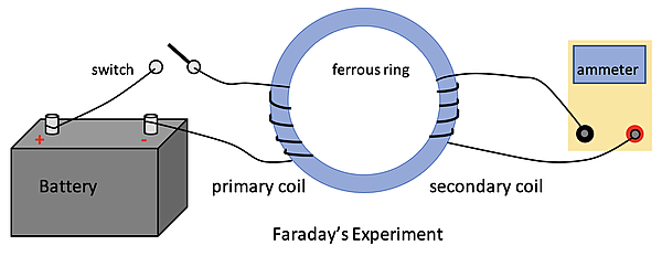
In the 1800’s Michael Faraday used the setup above to perform the following experiments:
An outline of the experiment Michael Faraday did in the 1800s
Action
Observation
Interpretation
1: Close the Switch
A temporary current is measured in the secondary coil before returning to 0.
Current set up in the primary coil builds up a magnetic field around the wire in the ring.
2: Switch stays closed.
The ammeter reading stays at 0.
Current in the primary coil and the magnetic field stays fixed at the same nonzero magnitude.
3: Open the switch
A temporary current is measured in the secondary coil in the opposite direction of Action 1 before returning to 0.
Current in the primary coil is halted, causing the magnetic field around the wire and in the right to drop to 0.
4: Switch stays open.
The ammeter reading stays at 0.
Current in the primary coil and the magnetic field stay fixed at 0.
Because of the brief occurrences of current in the secondary coil, it was concluded that a changing magnetic field in the ring produced an electric field in the secondary coil as though a source of potential difference [referred to as an induced emf (electromotive force)] was connected to it for a short period of time.
To study this phenomenon, the Magnetic Flux, \(Φ_B\), that is a measure of the strength of the magnetic field, \(B\), passing through a specific cross-sectional area, \(A\), is defined. It can be written as
\(Φ_b = B_\text{perpendicular} \times A = B \times A \times \cos{θ}\)
SI Unit: Weber (Wb)
\(B_\text{perpendicular}\) is the component of \(B\) perpendicular to the plane of the loop as shown below.
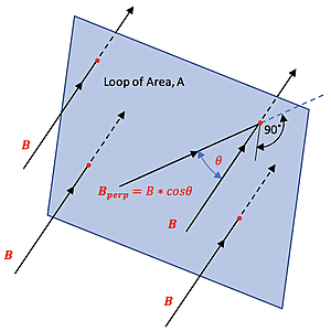
\(B_\text{perp} = B \times \cos{θ}\)
Faraday's Law of Induction
It has been determined that an emf (electromotive force) is induced in a circuit whn the magnetic flux through the circuit changes with time. The relationship between the change in flux and the emf is referred to as Faraday’s law of Magnetic Induction and written as follows:
\(ε = -N \times \frac{\delta Φ_B}{\text{δt}}\)
where \(N\) would be the number of tightly wound loops that experience the change in magnetic flux, \(\delta Φ_B\), during the time interval, \(\text{δt}\). The negative sign is used to determine the polarity of the induced emf. This is determined using Lenz’s Law stated as follows:
Lenz’s Law: The current caused by the induced emf travels in the direction that creates a magnetic field with flux opposing the change in the original flux through the circuit.
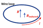
The creation of an emf due to a decreasing B-field is described in the table below:
Shows the electromagnetic field induced when a b-field is decreasing through a loop.
Situation
Diagram
Wire loop arranged horizontally with constant B-field pointing upwards.
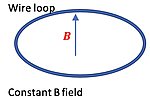
At a certain point in time the B-field starts decreasing
*Faraday's Law says that an emf will be established in the loop such that current will exist due to the changing B-field.
Lenz's Law says that the current will go in the direction shown using the right-hand rule to produce an induced B-field upwards that would oppose the change in the original B-field.
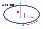
The creation of an emf due to an increasing B-field is described in the table below:
Shows the electromagnetic field induced when a b-field is decreasing through a loop.
Situation
Diagram
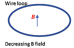
Wire loop arranged horizontally with constant B-field pointing upwards.
At a certain point in time the B-field starts increasing
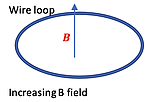
*Faraday's Law says that an emf will be established in the loop such that current will exist due to the changing B-field.
Lenz's Law says that the current will go in the direction shown using the right-hand rule to produce an induced B-field downwards that would oppose the change in the original B-field.
The creation of an emf due to a moving conductor and/or changing area in a magnetic field is called Motional emf. Let’s look at 2 scenarios below.
Scenario 1: Moving conductor
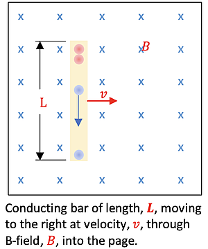
Conducting bar moving in a magnetic field as shown at right. A force due to the motion of charged particles is exerted on the charges in the bar, \(F = q \times v \descriptive{\text{ X }}{times, cross product} B\), causing a separation of charge by forcing negative electrons to move to the bottom of the bar according to the right-hand rule. This sets up an electric field pointing downwards in the conductor. Charge stops moving in the bar when the force due to the electric field matches the opposing force due to the magnetic field. Therefore, \(F_e = F_B\), and with substitution becomes \(q \times E = q \times v \times B\), giving \(E = v \times B\).
Like the capacitor, the potential difference (in this case the emf) set up by the separation of charge for the uniform electric field is \(E \times L\), so that the emf is the following:
\(ε = B \times L \times v\)
Scenario 2: Changing Area
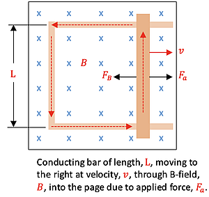
Consider a conducting bar experiencing an applied force, \(F_a\), to the right in a magnetic field as shown at right/above. A force due to the motion of charged particles is exerted on the charges in the bar, \(F = q \times v \descriptive{\text{ X }}{times, cross product} B\), causing a counterclockwise conventional current in the closed conductive pathway by the dotted red lines. The continual movement of the charge upwards in the moving bar causes the bar to experience a force, \(F_B\), to the left due to \(F = q \times v \descriptive{\text{ X }}{times, cross product} B\), applying the right-hand rule.
Therefore, an induced emf will be set up to oppose this increasing area and can be calculated using a change in Magnetic Flux. Consider the change in area shown below with the bar covering a distance, \(\text{δx}\),in a time of \(\text{δt}\).
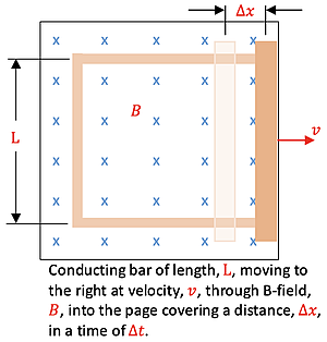
Using Faraday’s Law of Induction
\(ε = -N \times \frac{\delta Φ_B}{\text{δt}}\)
where \(N = 1\) becomes
\(ε = \frac{B \times \text{δtA}}{\text{δt}}\)
and since \(\text{δA} = L \times \text{δx}\),
\(ε = - \frac{B \times l \times \text{δx}}{\text{δt}}\)
and since \(v = \text{δx} \div \text{δt}\), then the magnitude of the emf is:
\(ε = B \times L \times v\)
Equation Summary
Summary of the Equations on this page
Concept
Equation
Magnetic Flux
\(Φ_b = B_\text{perpendicular} \times A = B \times A \times \cos{θ}\)
Faraday's Law
\(ε = -N \times \frac{\delta Φ_B}{\text{δt}}\)
Motion Emf
\(ε = B \times L \times v\)
Habits of an Effective Problem-Solver
An effective problem solver by habit approaches a physics problem in a manner that reflects a collection of disciplined habits. While not every effective problem solver employs the same approach, they all have habits which they share in common. These habits are described briefly here. Effective problem-solvers ...
- ...read the problem carefully and develops a mental picture of the physical situation. If needed, they sketch a simple diagram of the physical situation to help visualize it.
- ...identify the known and unknown quantities in an organized manner, often times recording them on the diagram itself. They equate given values to the symbols used to represent the corresponding quantity (e.g., \(F = \units{0.025}{N}\), \(E = 4.50 \times \units{10^{-6}}{\unitfrac{N}{C}}\), \(q = \colorbox{gray}{Unknown}\)).
- ...plot a strategy for solving for the unknown quantity. The strategy will typically center around the use of physics equations and is heavily dependent upon an understanding of physics principles.
- ...identify the appropriate formula(s) to use, often times writing them down. Where needed, they perform the needed conversion of quantities into the proper unit.
- ...perform substitutions and algebraic manipulations in order to solve for the unknown quantity.