Equation Overview - Magnetic Fields and Electromagnetism
Originally this section of Magnetism and Electromagnetic Induction were one page. We have split it to cover the Unit Magnetic Fields and Electromagnetic, and the unit Electromagnetic Induction separately. If you are on this page and looking for equations for Magnetic Flux or Faraday's Law of Induction, please see Electromagnetic Induction Equation Overview.
Problem Set Overview
We have 7 problem sets on the topic of Electromagnetism. Most problems are multi-part problems requiring an extensive analysis. The problems target your ability to apply concepts of electric circuits and magnetic fields in order to analyze situations in which a moving charge induces a magnetic effect.
The Origin of Magnetic Fields and Forces
Magnetic fields are produced by certain elements in nature. There are 4 levels of scale from smallest to largest that the element must satisfy for the object to display a magnetic field around it: 1) particle, 2) atom, 3) crystal structure, 4) domain.
Charged Particle:
Electrons orbiting the nucleus are tiny magnets due to their motion and a quantum property called spin. It gives the particle a tiny magnetic field called a magnetic moment. In a broader sense, spin is an essential property influencing the ordering of electrons and nuclei in atoms and molecules. The spin state can be either up or down. Protons also have the magnetic property of spin, but it is about 1000 times less in magnitude compared to the electron’s spin.Atom:
Atoms have many electrons orbiting the nucleus that fill orbitals. Electrons in a specific orbital pair up and in general, each electron pair consists of an up and a down spin characteristic that cancels out any overall magnetic effect. Therefore, atoms with half-filled outer shells have the best chance of being effectively magnetic.Crystal Structure:
Many elements form solids with atoms arranged in a crystal structure. This is defined as a particular repeating arrangement of atoms (molecules or ions) throughout the element. The atoms will arrange in a way that requires the lowest amount of energy, making it the most stable. In most of these arrangements the magnetic fields will be minimized.Domain:
Materials are made of sections of atoms with magnetic fields aligned. These sections are called domains. When one particular domain direction dominates the material, it will exhibit the physical characteristic of magnetism on a large scale.
Analyzing the periodic table and considering these 4 conditions, only iron, cobalt, and nickel are naturally occurring magnets at room temperature.
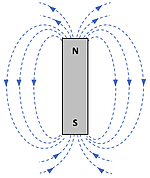
Any object able to create a magnetic field has polarity, producing north and south poles. Bar magnets create magnetic fields by having opposite poles (north and south) as shown below. The direction of the field is the direction the north pole of a compass needle points at that location.
If 2 poles are sufficiently small and far apart, they can be considered point magnetic charges. The force between 2 magnetic points is much like the Coulomb Force Law between charges and Newton’s Universal Law of Gravity between masses:
\(\descriptive{F_m}{F sub m, Force of magnetism} = K_m \times \frac{p_1 \times p_2}{\descriptive{r}{r, radius}^2}\)
where \(p_1\) and \(p_2\) are the magnitudes of the magnetic charges.
SI unit: \(\text{Ampere} \times \text{meter}\)
In this case,
\(K_m = \frac{μ}{4 \times π}\)
where \(µ = 4 \times π \times \units{10^{-7}}{\unitfrac{\descriptive{T}{T, Tesla}}{\descriptive{m \div A}{m slash a, meter ampere}}}\) and is the permeability of the intervening medium.
SI unit: \(\text{Tesla} \times \text{meter} \div \text{Ampere}\)
There is rarely a scenario where this is the case since monopoles don’t exist in nature. Complicated calculations have been developed for more common situations such as the force between 2 nearby magnetized surfaces, 2 nearby bar magnets, or 2 nearby cylindrical magnets. These situations are beyond the scope of these problems. A more common and useful way to produce a magnetic field is to set up a current in a wire. This magnetic field is observed since the current can put a force on a nearby magnet or moving charge.
Is Magnetic Field Fundamental?
There is disagreement about whether the Magnetic Field is fundamental to nature since the magnetic field can be viewed as an Electric Field in a certain frame of reference. This is like the "centrifugal" force and "Coriolis" force in that these forces are only observed in a specific (non-inertial) frame of reference.
Claim 1: The magnetic field is not fundamental and that can be seen when investigating the magnetic field created by a current. Let’s look at how a charge is affected by the current in a wire in the table below from the frame of reference of the charged particle outside the wire.
Case I: If the charged particle is not moving the equal number of protons and moving electrons equally spaced in the wire produce a net electric field of 0, thereby not affecting any nonmoving charged particles.
Case II & III: If the charged particle is moving parallel to the current then the concept of Special Relativity becomes relevant. In relative motion between the charged particle and the charges in the wire, the charge and quantum spin of any of the particles does not change (invariant). But what can change due to the relative motion between the charged particle and the charges in the wire (from the frame of reference of the charged particle) is space (length, distance, area, volume) among other physical characteristics.
Consider the following cases in the frame of reference of the positively charge particle:
An analysis of the 3 cases that support the claim that the magnetic field is not fundamental.
Case I:
Proton at rest relative to the positive nuclei in the wire.
Even distribution of charge in the wire, \(\text{E-Field} = 0\). The space between electrons is not moving relative to the resting particle so the wire remains neutral.
Case II:
Proton moving parallel to the electron flow in the same direction in a wire.
The E-Field is generated in the frame of reference of the moving particle due to the greater length contraction between positive nuclei of the atoms making up the metal wire. This creates a greater density of positive charge..
Case III:
Proton moving parallel to the electron flow in the opposite direction in a wire.
The E-field is generated in the frame of reference of the moving particle due to the lesser length contraction between the positive nuclei of the atoms making up the metal wire. The greater relative velocity of the electrons creates a greater density of negative charge..
Claim 2: The Magnetic Field is fundamental as best stated by Dr. Christopher S. Baird of West Texas A&M University below:
The correct statement is that electric fields and magnetic fields are both fundamental, both are real, and both are part of one unified entity: the electromagnetic field. Depending on what reference frame you are in, a particular electromagnetic field will look more electric and less magnetic, or more magnetic and less electric. However, this does not change the fact that they are both fundamental and both part of the same unified entity. A purely electric field as viewed in one inertial frame is part electric and part magnetic in all other reference frames. Similarly, a purely magnetic field as viewed in one inertial frame is part electric and part magnetic in all other reference frames. The magnetic field is not just a relativistic version of the electric field, and the electric field is not just a relativistic version of the magnetic field. Rather, the unified electromagnetic field is innately and self-consistently relativistic.
Though the generation of the magnetic field at the atomic level is complex we can analyze and make use of the behavior at the human scale and in the human frame of reference. The outcomes that we are concerned with are the following:
- A current (moving charge) in a wire produces a magnetic field around the wire.
- A stationary charged particle is not affected by a magnetic field.
- A moving charged particle feels a force from a magnetic field.
The Magnetic Field Definition due to a Magnetic Force
It is found experimentally that the strength of the magnetic force on a moving charged particle is proportional to the magnitude of the charge, \(q\) , the magnitude of the velocity \(v\), the strength of the external magnetic field, \(B\), and the sine of the angle, θ, between the direction of \(v\) and \(B\) as shown at right. This can be written as a cross product between \(v\) and \(B\):
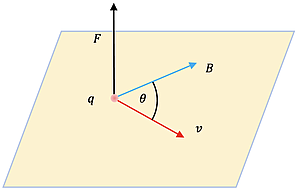
\(F = q \times v \descriptive{\text{ X }}{times, cross product} B = q \times v \times B \times \sin(θ)\)
This expression is rearranged to define the magnitude of the magnetic field as the following:
\(B = \frac{F}{qv \times \sin(θ)}\) SI unit: Tesla
The direction of the magnetic field is determined by the right-hand rule as shown in the diagram.
The Magnetic Force on a Current in a Wire
The magnitude of the force from a magnetic field on a current in a wire can be analyzed by rewriting the equation for Force from the reference frame of a point in the wire where \(L\) is the length of the wire, \(\text{δq} \div \text{δt}\) is the charge flow and \(B\) is the magnetic field as shown at right as follows:
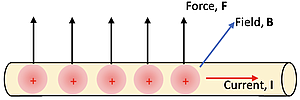
\(F = L \times \frac{\text{δθ}}{\text{δt}} \descriptive{\text{ X }}{times, cross product} B = L \times I \descriptive{\text{ X }}{times, cross product} B = L \times I \times B \times \sin{θ}\)
where \(I\) is the current in the wire and the direction is determined by the right-hand rule between conventional current, \(I\), and magnetic field, \(B\).
The Magnetic Force on the Current in a Loop
The previous result can be used to analyze the force on a current in the shape of a rectangular loop as shown below.
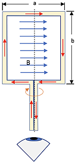
The current in the top and bottom sides of the loop is parallel to the \(B\)-field so the force from
\(F = a \times I \descriptive{\text{ X }}{times, cross product} B = a \times I \times B \times \sin{0°} = 0\)
The current in the left and right sides of the loop is perpendicular to the B-field so the result from \(F = b \times I \descriptive{\text{ X }}{times, cross product} B\) is
\(F = b \times I \times B \times \sin{90°} = b \times I \times B\)
The direction is obtained from the right-hand rule for cross products. The resulting forces are shown below from the eye’s view looking at the edge of the loop from the end position:
Since the forces do not go through the center of the loop a torque is produced that causes the loop to rotate about the center axis. The edge view reveals that the angle between the plane of the loop and the B-field, \(α\), changes over time as shown below.
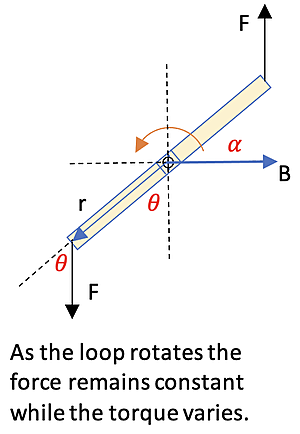
The torque at any loop position about the center axis due to one force will be \(τ = r \descriptive{\text{ X }}{times, cross product} F\). Since \(r = a \div 2\), \(F = b \times I \times B\) from above, and there are 2 identical forces, the net torque will be
\(\descriptive{τ}{tau, torque} = 2 \times ( \frac{a}{2} \times F \times \sin{θ} ) = a \times b \times I \times B \times \sin{θ}\)
When the loop is horizontal \(θ = 90°\), making the net Torque value a maximum of \(τ_\text{max} = a \times b \times I \times B\).
A Magnetic Force Outcome; Hall Effect
When a flow of electrons moves through a wire in a magnetic field the charges are separated in the wire by the right-hand rule of \(F = q \times v \descriptive{\text{ X }}{times, cross product} B\), where \(v\) is the drift velocity shown at right. This force on the electrons moves the negative charges to the bottom leaving positive charges near the top. This charge separation then sets up an E-field directed downward (called the Hall field) that puts a force on the moving electrons upward.
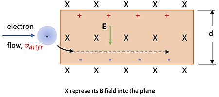
Establishing equilibrium between these 2 forces produces the following relationship:
\(F_\text{net} = 0 = q \times E_\text{Hall} - q \times v_\text{drift} \times B\)
and rearranging gives
\(E_\text{Hall} = v_\text{drift} \times B\)
From previous studies regarding separation of charge due to parallel plates the Potential Difference across the wire can be calculated by using \(\text{δV} = E \times d\). In this case, that Potential Difference is called the Hall emf:
\(\descriptive{ε_\text{Hall}}{epsilon sub hall, Hall emf} = E_\text{Hall} \times d = v_\text{drift} \times B \times d\)
A Magnetic Force Outcome; Mass Spectrometry
A flow of ions can be accelerated to a velocity, \(v\), and sent through a set of parallel plates as shown below.
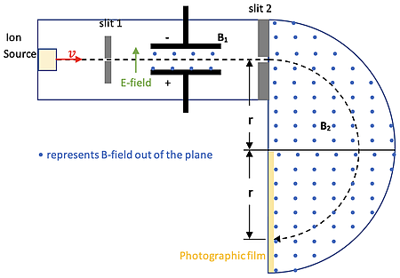
Opposing forces from the E-field and B-field are established with only ions having a certain velocity going straight through (\(F_\text{net} = 0\)) due to the relationship:
\(q \times E = q \times v \times B_1\)
and rearranging gives
\(v = \frac{E}{B_1}\)
These ions then enter another area having a magnetic field where they experience Uniform Circular Motion. Newton’s 2nd Law gives the following result:
\(F = q \times v \times B_2 = \frac{m \times v^2}{r}\)
Rearranging gives
\(\frac{q \times B_2 \times r}{v} = m\)
and substituting for \(v\) gives
\(m = \frac{q \times B_1 \times B_2 \times r}{E}\)
This result can be used to measure the mass of the ion.
The Magnetic Field Determined using Ampere’s Law
In electrostatics a charge that feels a force in an electric field also produces an electric field. In the same way a moving charge in a wire that feels a force from a B-field also generates a B-field of its own. This B-field can be determined using calculus and Ampere’s Law for moving charges
\(\oint B \times d \times l = \descriptive{μₒ}{mu sub o, vacuum permeability} \times \descriptive{I_\text{enc}}{i sub enc, Current of enclosed}\)
The result for the current in the wire to the below using Ampere’s Law is the following:
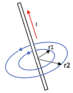
\(B = \frac{\descriptive{μₒ}{mu sub o, vacuum permeability} \times \descriptive{I_\text{enc}}{i sub enc, Current of enclosed}}{2 \times π \times r}\)
where \(µ_o = 4 \times π \times \units{10^{-7}}{t \times \unitfrac{m}{A}}\)
\(I_\text{enclosed}\) is the current in the wire, and
\(r\) is the distance from the wire to the location of interest.
The Magnetic Field created by the Current in a Solenoid
A long coil of wire consisting of many loops is called a solenoid as shown at right/below. Applying the right-hand rule to determine B-field lines when a current is sent through the wire gives the result that the B-field is reinforced in the center of the coil and not reinforced between the individual coils or immediately outside the coils.
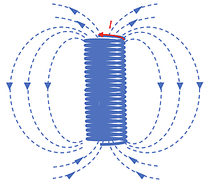
A solenoid acts like a bar magnet in that when current flows it has a north pole and a south pole, depending on the direction of the current. If the solenoid is very long in comparison to its diameter and the coils are tightly packed together, the field inside a solenoid is very nearly uniform in both direction and strength.
A solenoid cut in half with current shown in the coils is shown below.
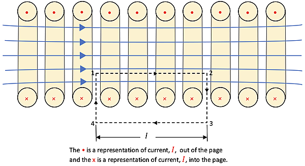
Ampere’s Law
\(\oint B \times d \times l = \descriptive{μₒ}{mu sub o, vacuum permeability} \times \descriptive{I_\text{enc}}{i sub enc, Current of enclosed}\)
can be used on a section of coils on one side of the solenoid as shown above using the dotted rectangle (\(N = \units{4}{\text{loops}}\)) to determine the magnitude of the B-field. The closed surface must be analyzed on all sides. Sides 2-3 and 4-1 are perpendicular to the B-field so no contribution will occur due to the dot product giving a \(\cos{90˚} = 0\). Side 3-4 has such a small B-field due to canceling effects from all coils so it will not contribute. The only side needing to be evaluated is side 1-2. The result is the following:
\(B \times L = \descriptive{μₒ}{mu sub o, vacuum permeability} \times \descriptive{I_\text{enc}}{i sub enc, Current of enclosed}\)
where \(\descriptive{I_\text{enc}}{i sub enc, Current of enclosed} = N \times I\),
\(µ_o = 4 \times π \times \units{10^{-7}}{t \times \unitfrac{m}{A}}\), and
\(L\) is the length of the rectangle
Therefore, the B-field produced by any solenoid can be calculated by using
\(B = \frac{\descriptive{μₒ}{mu sub o, vacuum permeability} \times N \times I}{L} = \descriptive{μₒ}{mu sub o, vacuum permeability} \times n \times I\)
where \(n = \frac{N}{L}\), the number of loops per unit length.
The Magnetic Field created by the Current in a Toroid
A long coil of wire consisting of many loops bent into the shape of a circle is called a toroid as shown below.
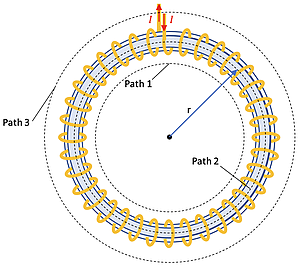
\(\oint B \times d \times l = \descriptive{μₒ}{mu sub o, vacuum permeability} \times \descriptive{I_\text{enc}}{i sub enc, Current of enclosed}\)
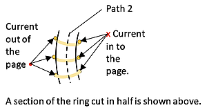
can be applied to the 3 pathways shown. Since there is no current inside Path 1 the B-field there is 0. Since the current flows into and out of the screen as shown at bottom right inside Path 3 the total current is 0 so the B-field there is 0.
Only in Path 2 do you get a current in one direction that qualifies for \(I_\text{enc}\) as part of Ampere’s Law. The result for Path 2 then will be the following:
\(B \times 2 \times π \times r = \descriptive{μₒ}{mu sub o, vacuum permeability} \times N \times I\)
where \(N \times I\) is the number of loops times the current.
The magnetic field is uniform within the toroid if the radius of the center of the ring, \(r\), is large relative to the width of the ring. Solving for the B-field magnitude then gives
\(B = \frac{\descriptive{μₒ}{mu sub o, vacuum permeability} \times N \times I}{2 \times π \times r} = \descriptive{μₒ}{mu sub o, vacuum permeability} \times n \times I\)
where \(n = N \div 2 \times π \times r\), the number of loops per unit length.
Equation Summary
A summary of the equations covered on this page.
Concept
Equation
Magnetic Force between 2 Magnetic Poles
\(\descriptive{F_m}{F sub m, Force of magnetism} = K_m \times \frac{p_1 \times p_2}{\descriptive{r}{r, radius}^2}\)
B-field Force on Moving Point Charge
\(F = q \times v \descriptive{\text{ X }}{times, cross product} B = q \times v \times B \times \sin(θ)\)
B-field Force on Current in a Wire
\(F = L \times I \descriptive{\text{ X }}{times, cross product} B = L \times I \times B \times \sin{θ}\)
Maximum Torque on Loop of Width a, and length b
\(τ_\text{max} = a \times b \times I \times B\)
Magnetic Force Outcome: Hall Effect
\(\descriptive{ε_\text{Hall}}{epsilon sub hall, Hall emf} = E_\text{Hall} \times d = v_\text{drift} \times B \times d\)
Magnetic Force Outcome: Mass Spectrometry
\(m = \frac{q \times B_1 \times B_2 \times r}{E}\)
B-Field using Ampere's Law
\(B = \frac{\descriptive{μₒ}{mu sub o, vacuum permeability} \times \descriptive{I_\text{enc}}{i sub enc, Current of enclosed}}{2 \times π \times r}\)
B-field for a Solenoid
\(B = \frac{\descriptive{μₒ}{mu sub o, vacuum permeability} \times N \times I}{L} = \descriptive{μₒ}{mu sub o, vacuum permeability} \times n \times I\)
B-field for a Toroid
\(B = \frac{\descriptive{μₒ}{mu sub o, vacuum permeability} \times N \times I}{2 \times π \times r} = \descriptive{μₒ}{mu sub o, vacuum permeability} \times n \times I\)
Habits of an Effective Problem-Solver
An effective problem solver by habit approaches a physics problem in a manner that reflects a collection of disciplined habits. While not every effective problem solver employs the same approach, they all have habits which they share in common. These habits are described briefly here. Effective problem-solvers ...
- ...read the problem carefully and develops a mental picture of the physical situation. If needed, they sketch a simple diagram of the physical situation to help visualize it.
- ...identify the known and unknown quantities in an organized manner, often times recording them on the diagram itself. They equate given values to the symbols used to represent the corresponding quantity (e.g., \(F = \units{0.025}{N}\), \(E = 4.50 \times \units{10^{-6}}{\unitfrac{N}{C}}\), \(q = \colorbox{gray}{Unknown}\)).
- ...plot a strategy for solving for the unknown quantity. The strategy will typically center around the use of physics equations and is heavily dependent upon an understanding of physics principles.
- ...identify the appropriate formula(s) to use, often times writing them down. Where needed, they perform the needed conversion of quantities into the proper unit.
- ...perform substitutions and algebraic manipulations in order to solve for the unknown quantity.