Equation Overview - Electric Circuits
NOTE: The original CalcPad unit for Electric Circuits was split into 4 subpages and had equations for 3 of the 4 sub sections. This is now combined onto this page. Please use the links below or the page level navigation to skip to the appropriate equations overview. Additionally, these pages existed before we had our Electric Circuit tutorials written, so the contents here go beyond a summary. We apologize for the length of this page.
Equation Overview - Electric Field, Potential, and Capacitance
Problem Set Overview
There are nine ready-to-use problem sets on the topic of Electrical Energy and Capacitors that are not reliant upon calculus. There are another six problem sets that are calculus-based. Most problems are multi-part problems requiring an extensive analysis. The problems target your ability to use the concepts of electric field, electric potential, electric potential energy, and electric capacitance to solve problems related to the interaction of charges with electrical fields.
Electric Fields
Fields of different types are all around us and are responsible for the behavior of matter/energy over time. A field is a physical quantity that has a value at each point in space. Some examples of fields:
- A source of heat creates a temperature field around it.
- A sink of heat creates a temperature field around it.
- A source of mass creates a gravitational field around it.
- A source of charge creates an electric field around it.
- A source of magnetism creates a magnetic field around it.
A certain characteristic of matter/energy reacts to these fields.
- Molecules can change their kinetic energy when placed in a temperature field.
- The physical characteristic of having mass means an object will experience a force when placed in a gravitational field.
- The physical characteristic of being charged means an object will experience a force when placed in an electric field.
- The physical characteristic of being magnetic means an object will experience a force when placed in a magnetic field.
- The physical characteristic of being a moving charge means an object will experience an electromagnetic force when placed in a magnetic field.
- The physical characteristic of having electron spin aligned means an object will experience an electromagnetic force when placed in a magnetic field.
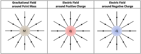
Due to their familiarity and similarity, we will begin by considering the gravitational field and the electric field which are both vector fields.
Any mass in the universe sets up a gravity field around it and any charged object sets up an electric field around it. Therefore, any object having mass will feel a force in the gravity field and any charged object or object able to be polarized will feel a force in an electric field.
These fields can be represented visually by lines with arrows indicating the direction of force on an object placed in the field as shown below. By convention the direction of the arrow in an electric field is determined by the direction of the force on a positive charge.
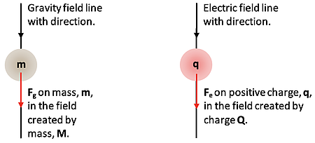
The field can be calculated by determining the force per unit of mass, \(m\), or unit of charge, \(q\), placed in the field. The gravity field value would be
\(g=\frac{F_g}{m}\)
and the electric field value would be
\(E=\frac{F_e}{q}\)
Diagrams of a single object experiencing a force in a field created by a single mass and a single charge.
Using Newton’s Universal Law of Gravity for \(F_g\), the gravity field value would be
\(g = \frac{\frac{G \times M \times m}{r^2}}{m} = \frac{G \times M}{r^2}\)
and using Coulomb’s Law for \(F_e\), the Electric field value would
\(E = \frac{\frac{k \times Q \times q}{r^2}}{q} = \frac{k \times Q}{r^2}\)
where \(M\) and \(Q\) are the physical characteristics of the objects creating the fields.
Analysis of Point Charges
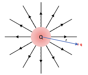
A point charge can be a single object of Charge, \(Q\). The object could also be a sphere or hollow shell of many charges that are distributed in different ways. If the object is conductive all the charges adding up to charge, \(Q\), are spread out on the outer surface. If the object is not conductive the charge could be spread throughout the object in various ways. No matter how the charge is distributed the electric field, \(E\), outside the object can be determined using the equation,
\(E = \frac{k \times Q}{r^2}\)
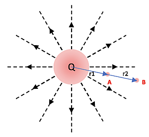
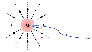
and its electric field lines will be radially configured as shown at right if the object is positive.
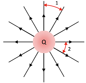
The radial lines have large distances between them as you get farther away from the center. This is an indication that the field is weaker. The comparison of spacing between E-field lines can be used to compare the strength of the field at various locations around a charged object. For example, Position 1 is at a weaker field location than Position 2.
When there are multiple E-Field sources in a region, the overall E-Field is the vector sum of E-fields from all sources. This is called The Principle of Superposition. The E-fields of all individual charges is calculated at a specific point and then replaced with the vector sum of these E-fields to get the overall E-field at this point.
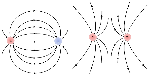
The diagrams below show the typical electric field line patterns that are obtained with 2 Point Charges.
Constant Electric Field
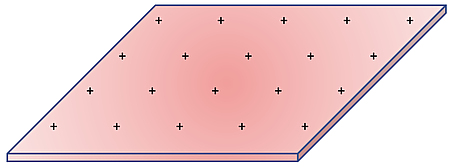
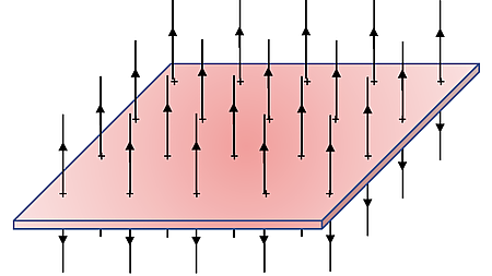
The value of E-fields created by a small number of separate charges is minimal due to the variable spacing of the field lines which means the magnitude of the field is different as you go from one position to another surrounding the charges. A valuable E-field would be one that was constant over a large area. This kind of E-field can be created by a thin, conductive plate uniformly charged as shown below.
The field lines would look like the following:
Gauss’s Law
\(\oint_{S} \vec{E} \times d \vec{A} = \frac{Q_{enc}}{ε_0}\)
and calculus can be used to show that the E-field on either side of a plate filled with total charge, \(Q_\text{enclosed}\), would give the following result for the field at every position near the plate:
Flat, thin plate E-field:
\(E = \frac{σ}{2 \times ε_0}\)
where \(ε_o\) is the permittivity of free space with a value of \(8.85418782 \times \units{10^{-12}}{\unitfrac{\text{farads}}{\text{meter}}}\) and \(σ\) is the charge density on the surface:
\(σ = \frac{Q_\text{enclosed}}{\text{Area}}\)
The permittivity is a measure of how dense of an electric field is "permitted" to form around an electric charge. It is related to the \(k\) in Coulomb’s Law as follows:
\(k \approx \frac{1}{4 \times π \times ε_0}\)
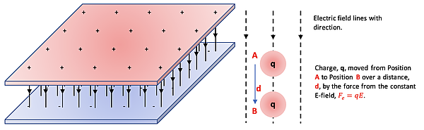
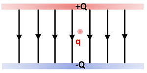
Two parallel plates close together of opposite charge \(Q\) and \(-Q\), would produce a field of twice the magnitude of a single plate as shown below.
Force of Electric Field: \(F_e = q \times E\)
Electric Field: $E = σ \div ε_0 $
Two flat, thin parallel plates of opposite charge E-field:
\(E = \frac{σ}{ε_0}\)
since the vector sum of each plate’s E-field adds between the plates and subtracts outside the plates. This electromechanical device is called a capacitor and one of its primary duties is to store charge, and therefore energy, in DC circuits.
Electric Potential Energy in Constant E-field
As with the gravitational force the electric force can do work on a charged object:
\(\text{Work}_\text{E-field} = F \times d = F_e \times d \times \cos{θ} = q \times E \times d\)
The change in Potential Energy of the charge produced by moving in the direction of the field can be written as:
\(\text{Work}_\text{E-field} = -\text{δPE} = \text{PE}_i - \text{PE}_f\)
and substituting from above gives
\(\text{δPE} = \text{PE}_f - \text{PE}_i = -{q \times E \times d}\)
Electric Potential Energy in E-field around a Point Charge
Consider a charge Q acting as a point charge and creating an electric field in the surrounding space.
The electric force can do work on a charged object, \(q\), in the field surrounding a Point Charge as shown at right. The issue here is that the E-field created by the charge, \(Q\), is not constant and has to be evaluated using calculus. The work done by the E-field on the moving charge from \(A\) to \(B\) is the following:
\(\text{Work}_{\text{E-field}} = \int_A^B F_e \times dr = \int_A^B q \times E \times dr \cos{θ} = \frac{q \times Q}{4 \times π \times ε_0} \int_A^B \frac{1}{r^2} \times dr\)
The result of the integration is the following:
\(\text{δPE} = \text{PE}_B - \text{PE}_A = -\text{Work}_{\text{E-field}} = \frac{q \times Q}{4 \times π \times ε_0} \left[ \frac{1}{r_2} - \frac{1}{r_1} \right]\)
The general expression for the Potential Energy of a charge, \(q\), a distance, \(r\), from the center of a charge, \(Q\), is determined as if the charge was moved by an outside force from a position of ∞:
\(\text{PE} = \text{PE}_r - \text{PE}_∞ = \frac{Q}{4 \times π \times ε_0} \left[ \frac{1}{r} - \frac{1}{∞} \right] = \frac{1}{4 \times π \times ε_0} \times (\frac{Q \times q}{r})\)
Electric Potential
In dealing with charged objects, it is valuable to work with the idea of Electric Potential Energy per Charge at a point in space in the Electric Field. The outcome of this ratio is that a relatively small charge at that position is not a factor as to the Potential of the field just like a relatively small charge at that position does not significantly affect the Electric Field. The concept of
\(\frac{\text{PE}}{q}\)
is called Electric Potential, \(V\). The Difference in Electric Potential between 2 points in an Electric Field is then:
\(\text{δV} = \frac{\text{δPE}}{q}\)
SI unit: Volts = J/C
Electric Potential for a Point Charge
For a position at distance, \(r\), from the center of a point charge, \(Q\), the Electric Potential at that point can be determined by considering moving the point charge, \(q\), in from \(∞\).
\(V = V_r - V_∞ = \frac{1}{q}(PE_r - PE_∞) = \frac{1}{q} \left[ \frac{q \times Q}{4 \times π \times ε_0} \left( \frac{1}{r} - \frac{1}{∞} \right) \right]= \frac{1}{4 \times π \times ε_0} \left( \frac{Q}{r} \right)\)
Electric Potential between Parallel Plates
When moving a charge, \(q\), a distance, \(d\), between parallel plates from Position A to Position B and since \(\text{PE}_A > \text{PE}_B\) the result is the following:
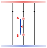
\(\text{δV}_{A \to B} = \frac{\text{δPE}_{A \to B}}{q} = \frac{-{q \times E \times d}}{q} = -{E \times d}\)
Equipotential Lines
Lines can be added to Electric Field diagrams that connect points of equal Electric Potential. This is useful to determine whether the Electric Potential Energy increases, decreases, or remains the same when a charge changes position. The single Point Charge Electric Field diagram is shown at right with blue circles added such that each line represents a set of positions of equal Electric Potential. These are called EquiPotential lines.
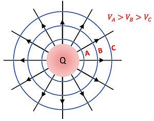
Voltage Comparison: \(V_A > V_B > V_C\)
The Equipotential Lines for a constant Electric Field between parallel plates are shown as blue lines below.
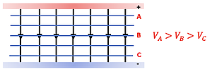
Voltage Comparison: \(V_A > V_B > V_C\)
The Equipotential Lines for an Electric Field created by opposite charges are shown as blue lines below.
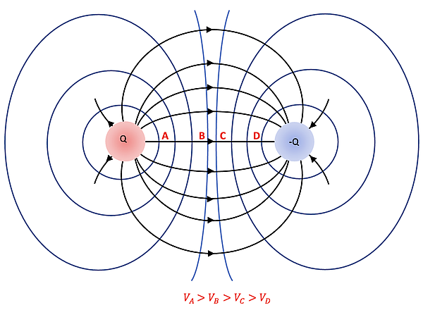
Voltage Comparison: \(V_A > V_B > V_C > V_D\)
Considerations when analyzing EquiPotential Lines:
- They are perpendicular to electric field lines since the value of the field does not change anywhere on the line.
- An outside force does positive work to move a positive charge against the field, say from Line C to Line A in the diagrams above, thereby increasing the Potential Energy of the charge and the Electric Potential at the charge’s new position in the field.
- An outside force does negative work to move a positive charge with the field, say from Line A to Line C in the diagrams above, thereby decreasing the Potential Energy of the charge and the Electric Potential at the charge’s new position in the field.
- An outside force does no work to move a positive charge perpendicular to the field, say from one position on Line B to another position on Line B in the diagrams above, thereby not changing the Potential Energy of the charge or the Electric Potential at the charge’s new position in the field.
The Capacitor
Characteristics:
- Generally made of 2 parallel metal plates.
- Made close enough together compared to the dimensions of the plates so that the E-field between the plates is constant.
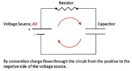
- When hooked up to a voltage source as shown below the capacitor will become charged over time ending with one positive plate and one negative plate having the same potential difference as the voltage source.
- The E-field set up between the plates is
\(E = \frac{σ}{ε_0}\)
- The E-field set up between the plates stores Electric Potential Energy.
Capacitance of a Capacitor
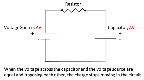
Charge stops flowing into and out of the plates of a capacitor when the Potential difference between the voltage source positive plate and the capacitor positive plate is equal to 0, and similarly the Potential difference between the voltage source negative plate and the capacitor negative plate is equal to 0.
After charging the following relationships for the capacitor are then established:
1: \(\text{δV}_\text{source} = \text{δV}_\text{plates} = E \times d\)
2: \(E = \frac{σ}{ε_0}\)
3: \(σ = \frac{Q}{A}\)
Substituting Equation 2 into Equation 1 gives
\(\text{δV} = \frac{σ}{ε_0} \times d\)
and then substituting Equation 3 in gives
\(\text{δV} = \frac{Q}{ε_0 \times A} \times d\)
and finally rearranging gives
\(\frac{ε_0 \times A}{d} = \frac{Q}{\text{δV}}\)
The amount of charge, \(Q\), able to be stored in a capacitor for a given Potential difference, \(\text{δθ}\), depends on the physical characteristics of the capacitor as shown by the left side of the previous equation. This is called the capacitance, \(C\), of the capacitor:
\(C = \frac{ε_0 \times A}{d}\)
The relationship between \(Q\), \(C\), and \(\text{δV}\) is therefore the following:
\(Q = C \times \text{δV}\)
Energy Stored in a Capacitor
Work is required to store positive and negative charges on the plates of a capacitor, thereby storing Potential Energy in the E-field between the capacitor plates.
A graph of the charge building up on the plates, \(Q\), versus time is shown at right/below. Below that is a graph of \(\text{δV}\) versus \(Q\) as the capacitor becomes fully charged.
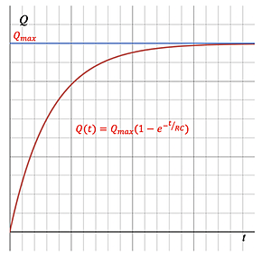
Capacitor Charge: \(Q(t) = Q_\text{max} \times (1 - e^{-t \div \text{RC}})\)
The bottom graph shows that as the charge, \(Q\), builds up on the plates the Potential difference between the plates, \(\text{δV}\), increases at a linear rate. The work done, and therefore the Potential Energy stored, is the area below the line. It can be represented 3 different ways using previous results:
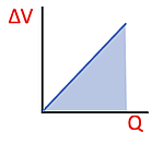
\(\text{Work} = \text{δPE} = \frac{1}{2} \times Q \times \text{δV} = \frac{1}{2} \times C \times \text{δV²} =\frac{1}{2} \times \frac{Q^2}{C}\)
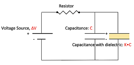
Dielectric in a Capacitor
A dielectric is an electrical insulator that can be polarized when placed in an E-field. When the dielectric material is sandwiched between 2 parallel plates as shown below right an additional, smaller E-field created by the polarized dielectric molecules is set up between the plates pointing in the opposite direction of the original E-field.
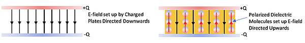
The vector sum of the 2 E-fields results in a smaller overall E-field between the plates. This reduces the voltage between the plates by a factor of \(K\), where \(K > 1\).
Without further charging and with the dielectric in place the capacitance would become
\(C_\text{dielectric} = \frac{Q}{(\frac{\text{δV}}{K})}\)
This would result in a capacitance of
\(C_\text{dielectric} = K \times \frac{Q}{\text{δV}} = K \times C\)
since
\(C = \frac{Q}{\text{δV}}\)
If the voltage source is charging with the dielectric in place more charge will be forced onto each plate as shown below until the voltage between the plates is equal to the source voltage, thereby storing more charge in the capacitor.
\(Q_\text{dielectric} = C_\text{dielectric} \times \text{δV}_\text{source}\)

Equation Summary
Situation: Point Charge
Concepts and Equations around Point Charge situations (small q going out from large Q point charge)
Concepts
Equation
E-field around source charge, uppercase Q
\(E = \frac{1}{4 \times π \times ε_0} \times \frac{Q}{r^2}\)
Force on test charge in field, lowercase q
\(F = q \times E = \frac{1}{4 \times π \times ε_0} \times \frac{q \times Q}{r^2}\)
Potential Energy of charge, lowercase q,
around source charge, uppercase Q.
\(\text{PE} = \frac{1}{4 \times π \times ε_0} \times (\frac{q \times Q}{r})\)
Electric Potential of charge, lowercase q,
around source charge, uppercase Q.
\(V = \frac{\text{PE}}{q} = \frac{1}{4 \times π \times ε_0} \times (\frac{Q}{r})\)
Situation: Constant Electric Field
Concepts and Equations around a Constant Electric Field
Concepts
Equation
E-field between plates.
\(E = \frac{σ}{ε_0}\)
Force on test charge, lowercase q, in field.
\(F = q \times E = \frac{q \times σ}{ε_0}\)
Change in Potential Energy of charge, lowercase q,
as it moves against E-field between plates.
\(\text{δPE} = q \times E \times d\)
Change in Potential of Charge, lowercase q, as it
moves against E-field between plates.
\(\text{δV} = \frac{\text{PE}}{q} = E \times d\)
Situation: Capacitors
Capacitance of Normal Capacitor: \(C\)
Capacitance of Dielectric Capacitor: \(K \times C\)
Concepts and Equations around Capacitor situations
Concepts
Equation
Capacitor Capacitance
\(C = \frac{ε_0 \times A}{d}\)
Charge stored in Capacitor
\(Q = C \times \text{δV}\)
Energy stored in Capacitor
\(½ \times Q \times \text{δV} = ½ \times C \times \text{δV²} = ½ \times \frac{Q^2}{C}\)
Capacitor Capacitance with Dielectric
\(C_\text{di} = K \times C = K \times \frac{ε_0 \times A}{d}\)
Habits of an Effective Problem-Solver
An effective problem solver by habit approaches a physics problem in a manner that reflects a collection of disciplined habits. While not every effective problem solver employs the same approach, they all have habits which they share in common. These habits are described briefly here. Effective problem-solvers...
- ...read the problem carefully and develops a mental picture of the physical situation. If needed, they sketch a simple diagram of the physical situation to help visualize it.
- ...identify the known and unknown quantities in an organized manner, often times recording them on the diagram itself. They equate given values to the symbols used to represent the corresponding quantity (e.g., \(F = \units{0.025}{N}\), \(E = 4.50 \times \units{10^{-6}}{\unitfrac{N}{C}}\), \(q = \colorbox{gray}{Unknown}\)).
- ...plot a strategy for solving for the unknown quantity. The strategy will typically center around the use of physics equations and is heavily dependent upon an understanding of physics principles.
- ...identify the appropriate formula(s) to use, often times writing them down. Where needed, they perform the needed conversion of quantities into the proper unit.
- ...perform substitutions and algebraic manipulations in order to solve for the unknown quantity.
Equation Overview - Electric Circuits
Problem Set Overview
There are 15 ready-to-use problem sets on the topic of Electric Circuits. The problems target your ability to use circuit concepts and equations to analyze simple circuits, series circuits, parallel circuits, and combination circuits. Problems range in difficulty from the very easy and straight-forward to the very difficult and complex.
Current
When charge flows through the wires of an electric circuit, current is said to exist in the wires. Electric current is a quantifiable notion that is defined as the rate at which charge flows past a point on the circuit. It can be determined by measuring the quantity of charge that flows past a cross-sectional area of a wire on the circuit. As a rate quantity, current (I) is expressed by the following equation
\(I = \frac{Q}{t}\)
where \(Q\) is the quantity of charge flowing by a point in a time period of \(t\). The standard metric unit for the quantity current is the ampere, often abbreviated as Amps or A. A current of 1 ampere is equivalent to 1 Coulomb of charge flowing past a point in 1 second. Since the quantity of charge passing a point on a circuit is related to the number of mobile charge carriers (electrons) which flow past that point, the current can also be related to the number of electrons and the time. To make this connection between the current and the number of electrons, one must know the quantity of charge on a single electron.
\(Q_\text{electron} = 1.6 \times \units{10^{-19}}{C}\)
Resistance
As charge flows through a circuit, it encounters resistance or a hindrance to its flow. Like current, resistance is a quantifiable term. The quantity of resistance offered by a section of wire depends upon three variables - the material the wire is made out of, the length of the wire, and the cross-sectional area of the wire. One physical property of a material is its resistivity - a measure of that material's tendency to resist charge flow through it. Resistivity values for various conducting materials are typically listed in textbooks and reference books. Knowing the resistivity value (ρ) of the material the wire is composed of and its length (\(L\)) and cross-sectional area (\(A\)), its resistance (\(R\)) can be determine using the equation below.
\(R = ρ \times \frac{L}{A}\)
The standard metric unit of resistance is the ohm (abbreviated by the Greek letter \(Ω\)).
The main difficulty with the use of the above equation pertains to the units of expression of the various quantities. The resistivity (ρ) is typically expressed in \(ohm \times m\) (Ohm meters). Thus, the length should be expressed in units of m and the cross-sectional area in \(m^2\). Many wires are round and have a circular cross-section. As such, the cross-sectional area in the above equation can be calculated from knowledge of the wire's radius or diameter using the formula for the area of a circle.
\(A = π \times R^2 = π \times \frac{D^2}{4}\)
Use our video on Electric Resistance to solidify your understanding of these resistance formulas.
Voltage-Current-Resistance Relationship
The amount of current that flows in a circuit is dependent upon two variables. Current is inversely proportional to the overall resistance (\(R\)) of the circuit and directly proportional to the electric potential difference impressed across the circuit. The electric potential difference (\(\text{δV}\)) impressed across a circuit is simply the voltage supplied by the energy source (batteries, outlets, etc.). For homes in the United States, this value is close to 110-120 Volts. The mathematical relationship between current (\(I\)), voltage (\(V\)) and resistance (\(R\)) is expressed by the following equation (which is sometimes referred to as the Ohm's law equation).
\(\text{δV} = I \times R\)
Power
Electrical circuits are all about energy. Energy is put into a circuit by the battery or the commercial electricity supplier. The elements of the circuit (lights, heaters, motors, refrigerators, and even wires) convert this electric potential energy into other forms of energy such as light energy, sound energy, thermal energy and mechanical energy. Power refers to the rate at which energy is supplied or converted by the appliance or circuit. It is the rate at which energy is lost or gained at any given location within the circuit. As such, the generic equation for power is
\(P = \frac{\text{δE}}{t}\)
The energy loss (or gain) is simply the product of the electric potential difference between two points and the quantity of charge which moves between those two points in a time period of t. As such, the energy loss (or gain) is simply \(\text{δV} \times Q\). When this expression is substituted into the above equation, the power equation becomes
\(P = \text{δV} \times \frac{Q}{t}\)
Since the \(Q \div t\) ratio found in the above equation is equal to the current (\(I\)), the above equation can also be written as
\(P = \text{δV} \times I\)
By combining the Ohm's law equation with the above equation, two other power equations can be generated. They are
\(P = I^2 \times R\) \(P = \frac{\text{δV}}{R}\)
The standard metric unit of power is the Watt. In terms of units, the Watt is equivalent to an \(\text{Amp} \times \text{Volt}\), an \(\text{Amp}^2 \times \text{Ohm}\), and a \(\text{Volt}^2 \div \text{Ohm}\).
Our video on Electric Power Equations will discuss these formulae in greater detail.
Electricity Costs
A commercial power company charges households for the energy supplied on a monthly basis. The bill for the services typically states the amount of energy consumed during the month in units of \(\text{kiloWatt} \times \text{hours}\). This unit - a power unit multiplied by a time unit - is a unit of energy. A household typically pays the bill on the basis of the number of \(kW•hr\) of electrical energy consumed during the month. Thus, the task of determining the cost of using a specific appliance for a specified period of time is quite straightforward. The power must first be determined and converted to kiloWatts. This power must then be multiplied by the usage time in hours to obtain the energy consumed in units of \(kW•hr\). Finally, this energy amount must be multiplied by the cost of electricity on a $ per kW•hr basis in order to determine the cost in dollars.
Equivalent Resistance
It is quite common that a circuit consist of more than one resistor. While each resistor has its own individual resistance value, the overall resistance of the circuit is different than the resistance of the individual resistors which make up the circuit. A quantity known as the equivalent resistance indicates the total resistance of the circuit. Conceptually, the equivalent resistance is the resistance that a single resistor would have in order to produce the same overall effect on the resistance as the combination of resistors that are present. So, if a circuit has three resistors with an equivalent resistance of 25 ohm, then a single 25-ohm resistor could replace the three individual resistors and have the equivalent effect upon the circuit. The value of the equivalent resistance (\(R_\text{eq}\)) takes into consideration the individual resistance values of the resistors and the way in which those resistors are connected.
There are two basic ways in which resistors can be connected in an electrical circuit. They can be connected in series or in parallel. Resistors that are connected in series are connected in consecutive fashion such that all the charge that passes through the first resistor will also pass through the other resistors. In series connection, all of the charge flowing through the circuit passes through each one of the individual resistors. As such, the equivalent resistance of series-connected resistors is the sum of the individual resistance values of those resistors.
\(R_\text{eq} = R_1 + R_2 + R_3 + \ldots \text{(series connection})\)
Resistors that are connected in parallel are connected in side-by-side fashion such that the charge approaching the resistors will split up into two or more different paths. Parallel-connected resistors are characterized as having branching locations where charge branches off into the different pathways. The charge which passes through one resistor will not pass through the other resistors. The equivalent resistance of parallel-connected resistors is less than the resistance values of all the individual resistors in the circuit. While it may not be entirely intuitive, the equation for the equivalent resistance of parallel-connected resistors is given by an equation with several reciprocal terms.
\(\frac{1}{R_\text{eq}} = \frac{1}{R_1} + \frac{1}{R_2} + \frac{1}{R_3} +\ldots \text {(parallel connections})\)
Series Circuit Analysis
Several of the problems in this unit pertain to series circuits. It is not unusual that a problem be accompanied by a drawing or a schematic diagram showing the arrangement of batteries and resistors. The drawing and corresponding schematic diagram below represents a series circuit powered by three cells and having three series-connected resistors (light bulbs).
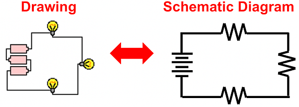
By imagining a charge leaving the positive terminal of the battery and following its path as it traverses the complete loop, it becomes evident that the charge goes through every resistor in consecutive fashion. As such it meets the criteria of a series circuit. Knowing that the circuit is a series circuit, allows you to relate the overall or equivalent resistance of the circuit to the individual resistance values by the equivalent resistance equation discussed above.
\(R_\text{eq} = R_1 + R_2 + R_3 + \ldots \text{(series connection})\)
The current of a series circuit is the same in the resistors as it is in the battery. Since there is no branching off locations where charge divides into pathways, it can be stated that the current in the battery is equal to the current in resistor 1 is equal to the current in resistor 2 and is equal to the current in resistor 3... In equation form, it can be written that
\(I_\text{battery} = I_1 = I_2 = I_3 = \ldots \text{(series circuit)}\)
As charge traverses the resistors of a series circuit, there is a drop in electric potential as it passes through each resistor. This drop in electric potential across each resistor is determined by the current through the resistor and the resistance of the resistor. This is consistent with the Ohm's law equation described above (\(\text{δV} = I \times R\)). Since the current (\(I\)) in each individual resistor is the same, it is logical to conclude that the resistors with the greatest resistance (\(R\)) will have the greatest electric potential difference (\(\text{δθ}\)) impressed across them.
The electric potential difference across the individual resistors of a circuit is often referred to as a voltage drop. These voltage drops of the series-connected resistors are mathematically related to the electric potential or voltage rating of the cells or battery which power the circuit. If a charge gains 12 volts of electric potential as it passes through the battery of an electric circuit, then it will lose 12 V as it passes through the external circuit. This 12 V drop in electric potential results from a series of individual drops in electric potential as it passes through the individual resistors of the series circuit. These individual voltage drops (electric potential difference) add up to give the total voltage drop of the circuit, in equation form, it can be said that
\(\text{δV}_\text{battery} = \text{δV₁} + \text{δV₂} + \text{δV₃} + \ldots \text{(series circuit)}\)
where \(\text{δV}_\text{battery}\) is the electric potential gained in the battery and \(\text{δV₁}\), \(\text{δV₂}\) and \(\text{δV₃}\) are the voltage drops (or electric potential differences) across the individual resistors.
A more detailed and exhaustive discussion of series circuits and their analysis can be found at The Physics Classroom Tutorial. And our videos on Series Circuit Relationships and Series Circuit Analysis will be very helpful.
Parallel Circuit Analysis
Several problems in this unit pertain to parallel circuits. Again, it is not unusual that a problem be accompanied by a drawing or a schematic diagram showing the arrangement of batteries and resistors. The drawing and corresponding schematic diagram below represents a parallel circuit powered by three cells and having three parallel-connected resistors (light bulbs).
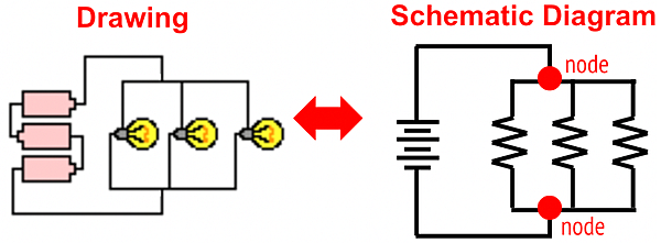
By imagining a charge leaving the positive terminal of the battery and following its path as it traverses the complete loop, it becomes evident that the charge reaches a branching location (a node) prior to reaching a resistor. At the branching location sometimes referred to as a node, charge follows one of the three possible paths through the resistors. Rather than pass through every resistor, a single charge will pass through a single resistor during a complete loop around the circuit. As such it meets the criteria of a parallel circuit. Knowing that the circuit is a parallel circuit, allows you to relate the overall or equivalent resistance of the circuit to the individual resistance values by the equivalent resistance equation discussed above.
\(\frac{1}{R_\text{eq}} = \frac{1}{R_1} +\frac{1}{R_2} +\frac{1}{R_3} + \ldots \text{(parallel connections)}\)
At the branching location, charge is splitting into separate pathways. As such, the current in the individual pathways will be less than the current outside the pathways. The overall current flow in the circuit and the current in the battery is equal to the sum of the current in the individual pathways. In equation form, it can be written that
\(I_\text{battery} = I_1 + I_2 + I_3 + \dots \text{(parallel circuits)}\)
The current values of these individual branches are controlled by two quantities - the resistance of the resistor in the branch and the electric potential difference (\(\text{δV}\)) impressed across the branch. Consistent with Ohm's law equation discussed above, it can be said that the current in branch 1 is equal to the electric potential difference across branch 1 divided by the resistance of branch 1. Similar statements can be made of the other branches. In equation form, it can be stated that
\(I_1 = \frac{\text{δV₁}}{R_1}\) \(I_2 = \frac{\text{δV₂}}{R_2}\) \(I_3 = \frac{\text{δV₃}}{R_3}\)
The electric potential differences (\(\text{δV₁}\), \(\text{δV₂}\) and \(\text{δV₃}\)) across the individual resistors are often referred to as voltage drops. Similar to series circuits, any charge leaving the battery must encounter the same drop in voltage as the gain that it encounters when passing through the battery. But unlike series circuits, a charge in a parallel circuit will only pass through one resistor. As such, the voltage drop across that resistor must equal the electric potential difference across the battery. In equation form, it can be stated that
\(\text{δV}_\text{battery} = \text{δV₁} = \text{δV₂} = \text{δV₃} = \ldots \text{(parallel circuits)}\)
where \(\text{δV}_\text{battery}\) is the electric potential gained in the battery and \(\text{δV₁}\), \(\text{δV₂}\) and \(\text{δV₃}\) are the voltage drops (or electric potential differences) across the individual resistors.
A more detailed and exhaustive discussion of parallel circuits and their analysis can be found at The Physics Classroom Tutorial. And our videos on Parallel Circuit Relationships and Parallel Circuit Analysis will be very helpful.
Habits of an Effective Problem-Solver
An effective problem solver by habit approaches a physics problem in a manner that reflects a collection of disciplined habits. While not every effective problem solver employs the same approach, they all have habits which they share in common. These habits are described briefly here. An effective problem-solver...
- ...reads the problem carefully and develops a mental picture of the physical situation. If needed, they sketch a simple diagram of the physical situation to help visualize it.
- ...identifies the known and unknown quantities and records them in an organized manner, often times recording them on the diagram itself. They equate given values to the symbols used to represent the corresponding quantity (e.g., \(\text{δV} = \units{9.0}{V}\); \(R = \units{0.025}{Ω}\); \(I = \colorbox{gray}{Unknown}\)).
- ...plots a strategy for solving for the unknown quantity; the strategy will typically center around the use of physics equations and be heavily dependent upon an understanding of physics principles.
- ...identifies the appropriate formula(s) to use, often times writing them down. Where needed, they perform the needed conversion of quantities into the proper unit.
- ...performs substitutions and algebraic manipulations in order to solve for the unknown quantity.
Additional Readings/Study Aids
The following pages from The Physics Classroom Tutorial may serve to be useful in assisting you in the understanding of the concepts and mathematics associated with these problems.
Watch a Video
We have developed and continue to develop Video Tutorials on introductory physics topics. You can find these videos on our YouTube channel. We have an entire Playlist on the topic of Electric Circuits.
Equation Overview - Transient RC Circuits
Problem Set Overview
We have four ready-to-use problem sets on the topic of Transient RC Circuits. Most problems are multi-part problems requiring an extensive analysis. The problems target your ability to apply concepts of potential, capacitance, resistance, and current in order to analyze transient RC circuits.
Electric Circuits
Circuit elements (Voltage sources, resistors, and capacitors) can be arranged into various configurations using conductive wires. The voltage across an element and the current in the element depend on the following principles and conventions.
- Positive charge will flow from high potential to low potential in a conductive circuit.
- Resistors can be assembled in series, parallel, and combination configurations.
- Resistor values are determined by physical characteristics: material, length, area.
- Capacitors can be assembled in series, parallel, and combination configurations.
- Capacitor values are determined by physical characteristics: dielectric, distance between plates, plate area.
- Once fully charged, capacitors act like an open in the circuit (no charge flow).
- When completely uncharged, capacitors act like a short in the circuit (unimpeded charge flow).
- Ohm’s Law and Kirchhoff’s Laws can be used to analyze circuit behavior.
Electric Circuit Schematic
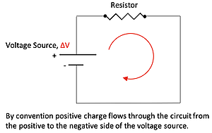
A simple circuit is shown at right. An individual resistor value can be calculated knowing the resistivity, length, and area of the resistor, \(R = ρ \times L \div A\). Current is the rate of charge flow, \(I = \text{δQ} \div t\). The voltage drop across the resistor will equal the Source Voltage and the current in the resistor can be calculated using Ohm’s Law, \(V = I \times R\). Power dissipated in the resistor can be calculated using any of the following expressions:
\(P = V \times I = \frac{v^2}{R} = I^2 \times R\)
Resistor Combinations

Two resistors in series give the following results.
- Equivalent resistance: \(R\text{eq} = R_1 + R_2\)
- Current: \(I_\text{total} = I_1 = I_2\)
- Voltage Drop: \(V_\text{total} = V_1 + V_2\)
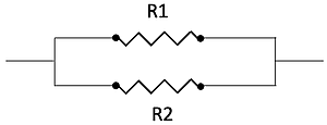
Two resistors in parallel give the following results.
- Equivalent resistance: \(R_\text{eq} = (R_1^{-1} + R_2^{-1})^{-1}\)
- Current: \(I_\text{total} = I_1 + I_2\)
- Voltage Drop: \(V_\text{total} = V_1 = V_2\)
Capacitor Charging
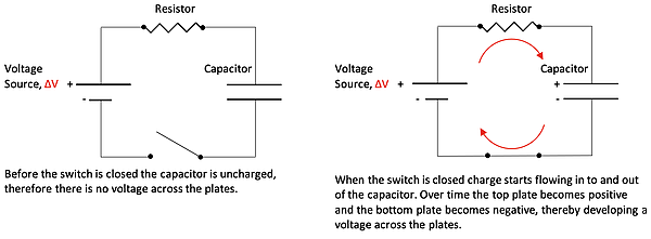
A capacitor can be wired in series with a resistor and voltage source to produce a resistor-capacitor (RC) circuit as shown below left. After closing the switch charge flow begins and produces a buildup of charge on the capacitor plates. The capacitor eventually causes the current to stop flowing in the circuit. This is because the charge buildup on the plates produces a voltage across the plates that is equal and opposing to the Voltage Source that originally moved the charge.
Kirchhoff’s Law and calculus can derive the charging equations for the RC circuit shown below.
Charge: \(Q(t) = Q_\text{max} \times (1 - e^{-t \div \text{RC}})\)
Voltage: \(V(t) = V_\text{max} \times (1 - e^{-t \div \text{RC}})\)
Current: \(I(t) = I_\text{max} \times e^{-t \div \text{RC}}\)
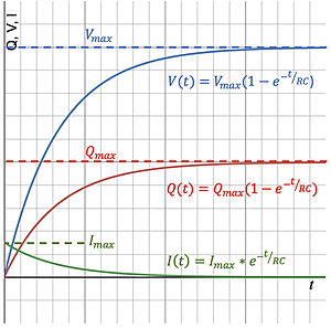
Those equations are shown with the associated curve at right. \(Q_\text{max}\) is the charge built up on the plates when the charging process is finished, \(V_\text{max}\) is the final voltage across the plates that develops due to the charge buildup, and \(I_\text{max}\) is the initial rate of charge flow. The time-based equations are:
- Amount of charge on the plates: \(Q(t) = Q_\text{max} \times (1 - e^{-t \div \text{RC}})\)
- Amount of voltage on the plates: \(V(t) = V_\text{max} \times (1 - e^{-t \div \text{RC}})\)
- Rate of charge flow in the circuit: \(I(t) = I_\text{max} \times e^{-t \div \text{RC}}\)
The relationship between the maximum values is the following:
\(Q_\text{max} = C \times V_\text{max}\), \(V_\text{max} = V_\text{source}\) and \(V_\text{source} = I_\text{max} \times R\)
Capacitor Discharging
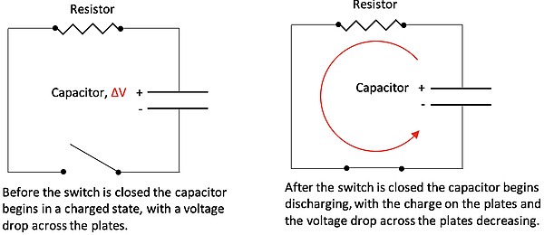
A charged capacitor can be wired in series with a resistor to produce the RC circuit as shown below left. After closing the switch, charge flow begins due to the Coulomb Force, thereby releasing the buildup of charge on the capacitor plates. The reduction in charge on the plates causes the voltage across the plates to decrease. This results in the charge on the plates, and the voltage drop across the plates to diminish to zero.
Kirchhoff’s Law and calculus can derive the discharging equations for the RC circuit shown below.
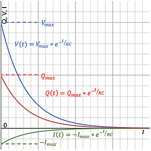
Charge: \(Q(t) = Q_\text{max} \times e^{-t \div \text{RC}}\)
Voltage: \(V(t) = V_\text{max} \times e^{-t \div \text{RC}}\)
Current: \(I(t) = -I_\text{max} \times e^{-t \div \text{RC}}\)
Those equations are shown with the associated curve at right. \(Q_\text{max}\) is the initial charge built up on the plates before the discharging process begins, \(V_\text{max}\) is the initial voltage drop across the plates that developed due to the charge buildup, and \(-I_\text{max}\) is the initial rate of charge flow. The negative sign indicates that the charge flow is in the opposite direction to the charge flow when charging the capacitor. The time-based equations are:
- Amount of charge on the plates: \(Q(t) = Q_\text{max} \times e^{-t \div \text{RC}}\)
- Amount of voltage on the plates: \(V(t) = V_\text{max} \times e^{-t \div \text{RC}}\)
- Rate of charge flow in the circuit: \(I(t) = -I_\text{max} \times e^{-t \div \text{RC}}\)
The relationship between the maximum values is the following:
\(Q_\text{max} = C \times V_\text{max}\) and \(V_\text{max} = I_\text{max} \times R\)
The Time Constant for RC Circuits
The multiplication of Resistance in Ohms multiplied by C in Farads results in a Time in Seconds. This product is referred to as the time constant, \(τ\), for the circuit whether it is charging or discharging:
\(τ = R \times C\)
For practical purposes a circuit is considered charged or discharged after a period of five time constants. Let’s look at an analysis of the voltage across the plates in a discharging capacitor at multiples of the time constant.
The time-based voltage equation for a discharging capacitor is: \(V(t) = V_\text{max} \times e^{-t \div \text{RC}}\)
Let’s substitute \(τ\) into the equation: \(V(t) = V_\text{max} \times e^{-t \div τ}\)
The voltage at \(t = 1 \times τ\): \(V(t) = V_\text{max} \times e^{-t \div τ} = V_\text{max} \times e^{-1} = 0.368 \times V_\text{max}\)
The voltage at \(t = 2 \times τ\): \(V(t) = V_\text{max} \times e^{-t \div τ} = V_\text{max} \times e^{-2} = 0.135 \times V_\text{max}\)
The voltage at \(t = 3 \times τ\): \(V(t) = V_\text{max} \times e^{-t \div τ} = V_\text{max} \times e^{-3} = 0.05 \times V_\text{max}\)
The voltage at \(t = 4 \times τ\): \(V(t) = V_\text{max} \times e^{-t \div τ} = V_\text{max} \times e^{-4} = 0.018 \times V_\text{max}\)
The voltage at \(t = 5 \times τ\): \(V(t) = V_\text{max} \times e^{-t \div τ} = V_\text{max} \times e^{-5} = 0.0067 \times V_\text{max}\)
The time-based voltage curves for the charging and discharging situations are shown below.
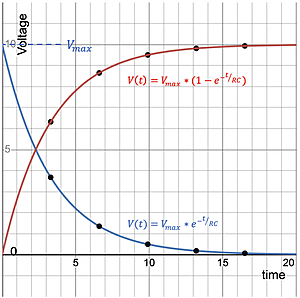
Charging: \(V(t) = V_\text{max} \times (1 - e^{-t \div \text{RC}})\)
Discharging: \(V(t) = V_\text{max} \times e^{-t \div \text{RC}}\)
The values for the voltage across the plates at the multiples of the time constant are plotted on the curves for the following values:
\(R = \units{1000}{Ω}\)
\(C = \units{3300}{\text{μf}}\)
\(τ = R \times C = \units{3.3}{s}\)
\(V_\text{max} = \units{10}{\text{Volts}}\)
Table showing the Time (in increments of tau) and the volts for charging and discharging
Time (sec)
V (Volts) - Charging
V (Volts) - discharging
\(1 \times τ = 3.3\)
6.32
3.68
\(2 \times τ = 6.6\)
8.65
1.35
\(3 \times τ = 9.9\)
9.50
0.50
\(4 \times τ = 13.2\)
9.82
0.18
\(5 \times τ = 16.5\)
9.93
0.067
Capacitor Combinations
Multiple capacitors can be arranged in circuits just like resistors; series, parallel, and a combination of the two.
Capacitors in Series: Let’s look at the charging of 2 identical capacitors in series compared to just 1 of them as shown in the circuits below.
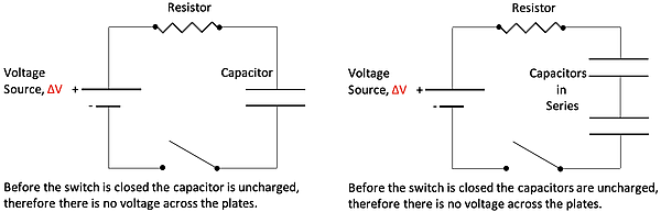
The circuits are shown below after the switch is closed and the capacitors are fully charged. Colored lines are used to represent the Electric Potential (Voltage) of the Voltage Source and the capacitors.
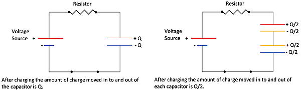
The voltage across the single capacitor is equal to the voltage source after charging. Due to Kirchhoff’s Voltage Law the voltage across an individual capacitor in the 2- capacitor circuit is half the voltage source. What does this say about the circuit overall capacitance? We can write the following equation after charge has stopped moving:
\(V_\text{across both caps} = V_1 + V_2\)
and since \(Q = C \times V\)
\(\frac{Q_\text{both caps}}{C_\text{both caps}} = \frac{Q_1}{C_1} + \frac{Q_2}{C_2}\)
and since \(V_\text{both caps} = V_1 = V_2\), the single capacitor that can replace two capacitors in series can be calculated by
\(\frac{1}{C_\text{equivalent}} = \frac{1}{C_1} + \frac{1}{C_2} = C_1^{-1} + C_2^{-1}\)
or
\(C_\text{equivalent} = (C_1^{-1} + C_2^{-1})^{-1}\)
Capacitors in Parallel: Let’s look at the charging of 2 identical capacitors in parallel compared to just 1 of them as shown in the circuits below.
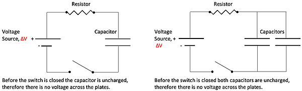
The circuits are shown below after the switch is closed and the capacitors are fully charged. Colored lines are used to represent the Electric Potential (Voltage) of the Voltage Source and the capacitors.
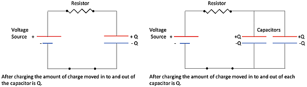
The voltage across the single capacitor is equal to the voltage source after charging. The voltage across an individual capacitor in the 2- capacitor circuit is also the same as the voltage source. What does this say about the circuit overall capacitance? We can write the following equation after charge has stopped moving:
\(Q_\text{into both caps} = Q_1 + Q_2\),
and since \(Q = C \times V\),
\(C_\text{equivalent} \times V_\text{source} = C_1 \times V_1 + C_2 \times V_2\)
and since \(V_\text{source} = V_1 + V_2\), the single capacitor that can replace two capacitors in parallel can be calculated by
\(C_\text{equivalent} = C_1 + C_2\)
Equation Summary
Resistors
Summary of the Concept and Equation for Resistors
Concepts
Equation
Resistance
\(R = \frac{ρ \times l}{A}\)
Resistors in Series
\(R_\text{eq} =\sum\limits_{i} R_i\)
Resistors in Parallel
\(\frac{1}{R_\text{eq}} =\sum\limits_{i} \frac{1}{R_i}\)
Voltage Source-Resistor DC Circuit
Summary of the Concept and Equation for Voltage Source-Resistor DC Circuit
Concepts
Equation
Current
\(I = \frac{\text{δQ}}{t}\)
Ohm's Law
\(V = I \times R\)
Power
\(P = V \times I = \frac{V^2}{R} = I^2 \times R\)
Capacitors
Summary of the Concept and Equation for Capacitors
Concepts
Equation
Capacitance
\(C = K \times ε_o \times \frac{A}{d}\)
Capacitors in Series
\(\frac{1}{C_\text{eq}} = \sum\limits_{i} \frac{1}{C_i}\)
Capacitors in Parallel
\(C_\text{eq} = \sum\limits_{i} C_i\)
Resistor-Capacitor RC Circuit
Summary of the Concept and Equation for Resistor-Capacitor RC Circuits.
Concepts
Equation
Charging
Charge \(Q(t) = Q_\text{max} \times (1 - e^{-t \div \text{RC}})\)
Voltage \(V(t) = V_\text{max} \times (1 - e^{-t \div \text{RC}})\)
Current \(I(t) = I_\text{max} \times e^{-t \div \text{RC}}\)
Discharging
Charge \(Q(t) = Q_\text{max} \times e^{-t \div \text{RC}}\)
Voltage \(V(t) = V_\text{max} \times e^{-t \div \text{RC}}\)
Current \(I(t) = -I_\text{max} \times e^{-t \div \text{RC}}\)
Time Constant
\(τ = R \times C\)
Habits of an Effective Problem-Solver
An effective problem solver by habit approaches a physics problem in a manner that reflects a collection of disciplined habits. While not every effective problem solver employs the same approach, they all have habits which they share in common. These habits are described briefly here. Effective problem-solvers ...
- ...read the problem carefully and develops a mental picture of the physical situation. If needed, they sketch a simple diagram of the physical situation to help visualize it.
- ...identify the known and unknown quantities in an organized manner, often times recording them on the diagram itself. They equate given values to the symbols used to represent the corresponding quantity (e.g., \(F = \units{0.025}{N}\), \(E = 4.50 \times \units{10^{-6}}{\unitfrac{N}{C}}\), \(q = \colorbox{gray}{Unknown}\)).
- ...plot a strategy for solving for the unknown quantity. The strategy will typically center around the use of physics equations and is heavily dependent upon an understanding of physics principles.
- ...identify the appropriate formula(s) to use, often times writing them down. Where needed, they perform the needed conversion of quantities into the proper unit.
- ...perform substitutions and algebraic manipulations in order to solve for the unknown quantity.